<?xml version="1.0" encoding="utf-8"?><feed xmlns="http://www.w3.org/2005/Atom" ><generator uri="https://jekyllrb.com/" version="4.1.1">Jekyll</generator><link href="https://oriont.net/feed.xml" rel="self" type="application/atom+xml" /><link href="https://oriont.net/" rel="alternate" type="text/html" /><updated>2025-12-21T21:55:57+00:00</updated><id>https://oriont.net/feed.xml</id><title type="html">oriont.net</title><subtitle>oriont.net holds information about projects created by oriont</subtitle><entry><title type="html">Games and Miscellaneous Projects</title><link href="https://oriont.net/posts/games" rel="alternate" type="text/html" title="Games and Miscellaneous Projects" /><published>2025-12-21T00:00:00+00:00</published><updated>2025-12-21T00:00:00+00:00</updated><id>https://oriont.net/posts/games</id><content type="html" xml:base="https://oriont.net/posts/games"><![CDATA[<p>A collection of small games and interactive projects I’ve built over the years, mostly using p5.js and vanilla JavaScript.</p>

<div class="flex flex-col space-y-6">
	<div>
		<a class="biglink" href="//oriont.net/solitaire">Solitaire</a>
		<p>My own implementation of classic solitaire in p5js.</p>
	</div>
    <div>
		<a class="biglink" href="//oriont.net/minesweeper">Minesweeper</a>
		<p>My implementation of classic minesweeper. It's configurable!</p>
	</div>
	<div>
		<a class="biglink" href="//oriont.net/gameoflife">Game of Life</a>
		<p>My implementation of Conway's Game of Life. It's rainbow!</p>
	</div>
	<div>
		<a class="biglink" href="//oriont.net/tone-wave">Tone Wave Simulator</a>
		<p>A simulation of a sinusoidal tone wave.</p>
	</div>
    <div>
		<a class="biglink" href="//oriont.net/maze-generator">Maze Generator</a>
		<p>A maze generator I made.</p>
	</div>
	<div>
		<a class="biglink" href="//oriont.net/sort-visualizer">Sort Visualizer</a>
		<p>A small sketch I made that visualizes different sorting algorithms in real time.</p>
	</div>
	<div>
		<a class="biglink" href="//oriont.net/pendulum">Double Pendulum</a>
		<p>My implementation of a double pendulum with a chaotic strange attractor visualization at the bottom.</p>
	</div>
	<div>
		<a class="biglink" href="//oriont.net/tetris">Tetris</a>
		<p>My implementation of tetris.</p>
	</div>
	<div>
		<a class="biglink" href="//oriont.net/unicode-generator">Unicode Generator</a>
		<p>A text scrambler.</p>
	</div>
	<div>
		<a class="biglink" href="//oriont.net/16-Hour-Project">16 Hour Project Grapher</a>
		<p>A 7th grade project where I made a bad desmos clone for only linear functions.</p>
	</div>
	<div>
		<a class="biglink" href="//oriont.net/2048">2048</a>
		<p>A clone of 2048 by Gabriele Circulli</p>
	</div>
	<div>
		<a class="biglink" href="//oriont.net/web-platformer">Web Platformer</a>
		<p>A small platformer engine made with javascript classes.</p>
	</div>
	<div>
		<a class="biglink" href="//oriont.net/MVCC-SpringContest">MVCC Spring Contest</a>
		<p>A small sketch depicting an environment as an entry for the MVCC Spring Contest.</p>
	</div>
</div>]]></content><author><name></name></author><category term="post" /><category term="games" /><summary type="html"><![CDATA[A collection of small games and interactive projects I’ve built over the years, mostly using p5.js and vanilla JavaScript.]]></summary></entry><entry><title type="html">Maximum Independent Set on Unit Disk Graph</title><link href="https://oriont.net/posts/misudg" rel="alternate" type="text/html" title="Maximum Independent Set on Unit Disk Graph" /><published>2024-10-30T00:00:00+00:00</published><updated>2024-10-30T00:00:00+00:00</updated><id>https://oriont.net/posts/misudg</id><content type="html" xml:base="https://oriont.net/posts/misudg"><![CDATA[<p>In this post I’ll share a practice exercise I got from my CS 4540 class at Georgia Tech and my solution to it.</p>

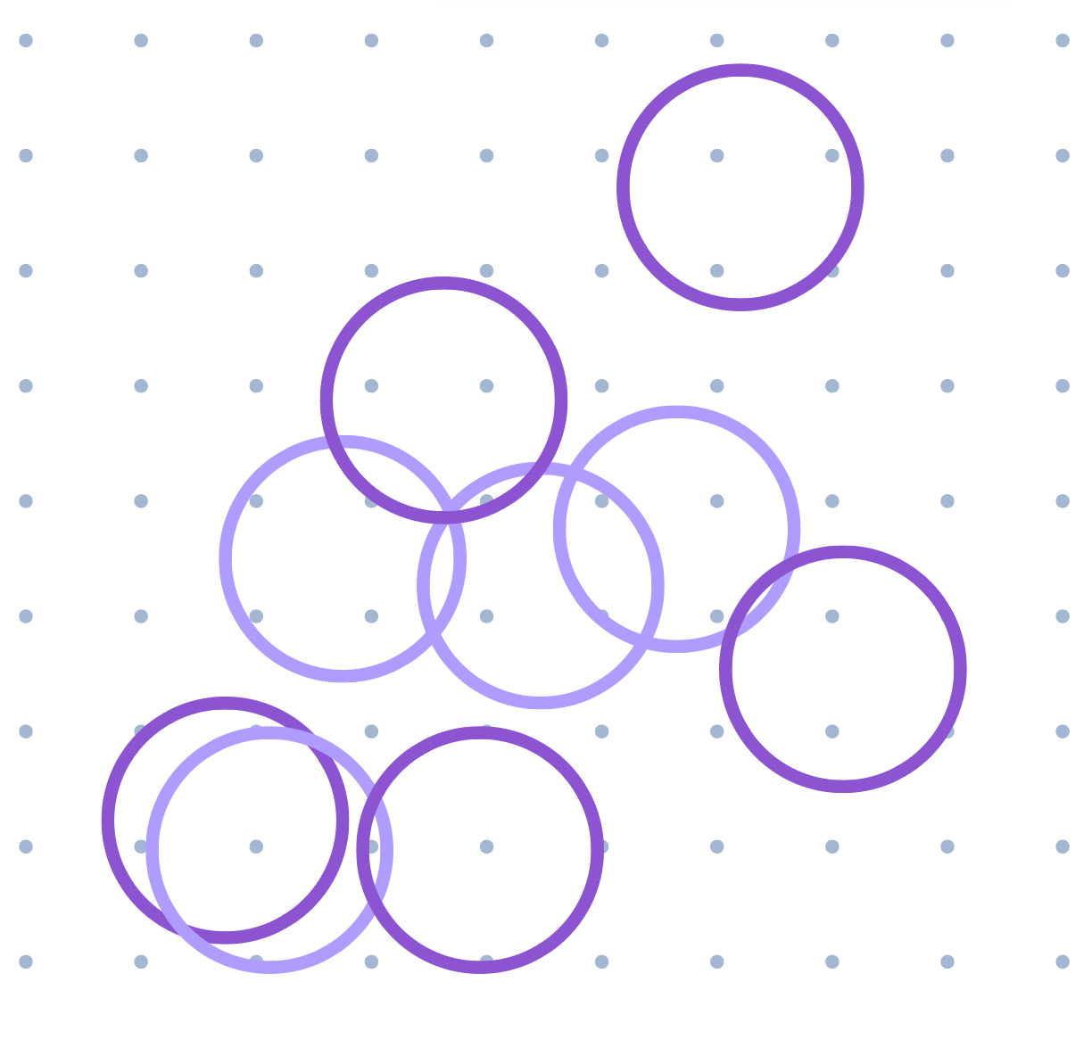
<p><img src="/assets/images/misudg/misudg_ex.jpeg" alt="MISUDG" /></p>

<h2 id="the-problem">The Problem</h2>
<p>In the Maximum Independent Set on Unit Disk Graph (MISUDG) problem, we are given a set \(S\) of unit-
diameter disks in the plane. The goal is to find a maximum-cardinality subset \(S' \subset S\) of disks, such that no
two disks in \(S'\) overlap. (We say that disks that only touch on the boundary do not overlap). As with the
Maximum Independent Set problem, this problem is also NP-Complete.</p>
<ol>
  <li>Consider the following greedy algorithm: start with \(S' = \varnothing\) and process the disks in S one by one,
in any order. For each such disk \(C\), if \(S' \cup C\) is a feasible solution, then add C to S′. What is the approxi-
mation factor of this algorithm? (Give the best upper bound you can.)</li>
  <li>Let \(0 &lt; \epsilon &lt; 1\) be some constant. Assume that we are given a grid whose lines are spaced \(\dfrac{1}{\epsilon}\) units
apart. Assume further that no disk in the input set S intersects the grid lines. Give a polynomial time
algorithm for solving the problem exactly in this case.</li>
  <li>Derive and analyze a PTAS for the MISUDG problem. <strong>Hint:</strong> Consider a grid with random offset:
Take a grid of lines spaced \(\dfrac{1}{2}\) apart, such that the origin is at the intersection of a horizontal and vertical grid
line. Pick a shift/offset \(L\) uniformly at random from \([0, \dfrac{1}{2})\), and shift the grid vertically and horizontally by
an distance \(L\). (Equivalently, consider the grid of spacing \(\dfrac{1}{2}\) such that the point \((L, L)\) is at the intersection
of two grid lines.) What is the probability that a disk is intersected by a grid line?</li>
</ol>

<h2 id="observe">Observe</h2>

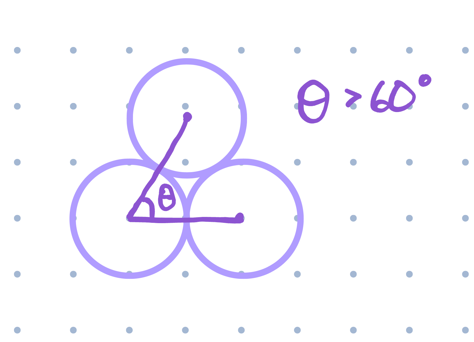
<p>We start out by noticing that for a disk \(x\), the maximum number of independent neighbors is 5.
This is because each neighbor must intersect \(x\), and the angle between the centers of neighbors must be greater than \(60^\circ\).
If \(\theta \leq 60\) then the neighbors would intersect eachother and wouldn’t be independent anymore, a contradiction.
Since there are \(360^\circ\) around \(x\), we have:</p>

\[360 = n (60 + \delta)\]

\[n &lt; 6\]

<p><img src="/assets/images/misudg/misudg_angle.jpeg" alt="Disk Angles" /></p>

<p>This means the <strong>maximum</strong> number of independent neighbors for <strong>any</strong> given disk is \(5\).</p>

<h2 id="solution-to-1">Solution to 1</h2>

<p>The greedy algorithm doesn’t choose disks in any particular order, so we choose the order it uses in the worst case scenario.
Notice for disk \(x\) with \(5\) independent neighbors, 2 maximal solutions would be either just disk \(x\), or all of the \(5\) independent neighbors.
(None of these neighbors intersect each other, so they would form an independent set.)</p>

<p>Let \(C^*\) be the largest independent set. 
For each disk \(d\), the worst possible case would be if instead of choosing \(d\), we chose its (up to) \(5\) independent neighbors.
Let \(C\) represent the greedy solution. 
So, we have \(|C| \leq 5 |C^*|\). 
This means greedy is a \(5\)-approximation of the optimal algorithm.</p>

<h3 id="remark">Remark</h3>

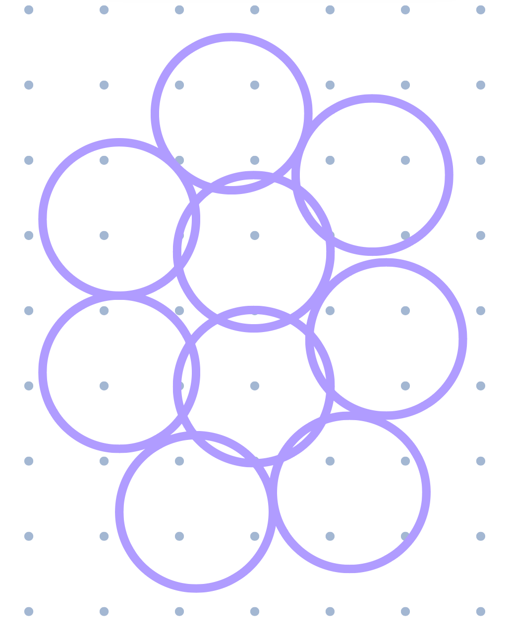
<p>Realistically, the actual approximation is a little better for larger input sets, since apart from this trivial case, not every disk in the optimal solution is surrounded by \(5\) independent disks. See the following picture for reference.</p>

<p><img src="/assets/images/misudg/misudg_stacked_disks.jpeg" alt="Stacked Disks" /></p>

<h2 id="solution-to-2">Solution to 2</h2>

<p>I thought this solution was pretty cool: we know independent set is NP-complete, so we can’t just convert to a graph and solve.
Instead, we do a crazy brute-force algorithm.</p>

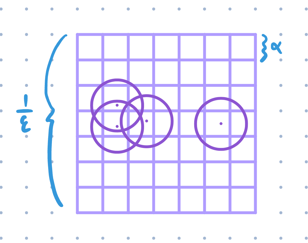
<p>Consider a single grid square of size \(\dfrac{1}{\epsilon} \times \dfrac{1}{\epsilon}\).
We split up this grid further into squares of size \(\alpha \times \alpha\). 
Each smaller square we assign the set of disks whose centers are contained within that square. 
(As an edge case, if a center is on the boundary, we just assign it to one of the squares.)</p>

<p>As long as we choose \(\alpha\) such that we can’t fit 2 disks next to each other without them intersecting in an \(\alpha \times \alpha\) square, we know at most 1 disk contained from this square will be in the independent set. 
(Since if there were 2, then they must intersect eachother, and therefore it wouldn’t be an independent set anymore)
We can choose \(\alpha = \dfrac{1}{\sqrt 2} - \delta\) since the longest distance in a square of side length \(\alpha\) is the diagonal of length less than \(1\).
If there were a disk on opposite corners, they must intersect since the radii are \(0.5\) but the distance between centers is less than \(1\). 
(We can set \(\delta=0\) for the purposes of the rest of the problem)</p>

<p><img src="/assets/images/misudg/misudg_small_grid.jpeg" alt="Smaller Grid" /></p>

<p>The actual independent set will contain 0 or 1 disk from each square–we know this because disks can still intersect across the little square boundaries, meaning we choose a disk from one little square but not the other. 
From this we can make a polynomial-sized list of candidates: we get every combination of 0 or 1 disk from each smaller square.
At most, there are \(n=|S|\) disks per smaller square. (Because what if all disks were in one square)
There are \(\dfrac{\dfrac{1}{\epsilon}}{\alpha}\) smaller squares per side of a larger square, giving us \(\dfrac{1}{(\epsilon \alpha)^2}\) total smaller squares per larger square.
This means there are at most \(n^\dfrac{1}{(\epsilon \alpha)^2}\) candidates to look through.
(We just take the number of combinations of the max number of disks in smaller square)</p>

<p>As large of a polynomial this is, it is still a polynomial, and we can loop through each candidate to check if it as an independent set, and find the largest one among those which are.
This is a polynomial way of getting the independent set for one square–we know the max independent set will be the union of all the max independent sets of the grid squares. 
(Since no disk can intersect across larger squares, we don’t have to worry about trying each candidate!)
Thus we have a polynomial time algorithm to give us an exact answer!</p>

<h3 id="remark-1">Remark</h3>

<p>Theoretically, and perhaps impractically (although this entire solution is impractical) we could do away with the larger grid and solve the entire problem exactly using the smaller grid squares. This would result in a much larger polynomial than we already had, but would still work. 
Also, the big grid square probably won’t divide \(\alpha\) evenly. This is fine, as we only really care about being able to iterate over <strong>space</strong> (which is polynomial) rather than <strong>vertex combinations</strong> (which is exponential).</p>

<h2 id="solution-to-3">Solution to 3</h2>

<p>We make the bigger grid and shift it by \(L\). 
We remove each disk that intersects a bigger grid line, and run the algorithm outlined in part 2 on this new set, giving us an approximation of the independent set. 
For the approximation ratio, we consider which disks we remove (which disks intersect the grid line).</p>

<p><img src="/assets/images/misudg/misudg_bigger_smaller.jpeg" alt="Bigger/Smaller square" /></p>

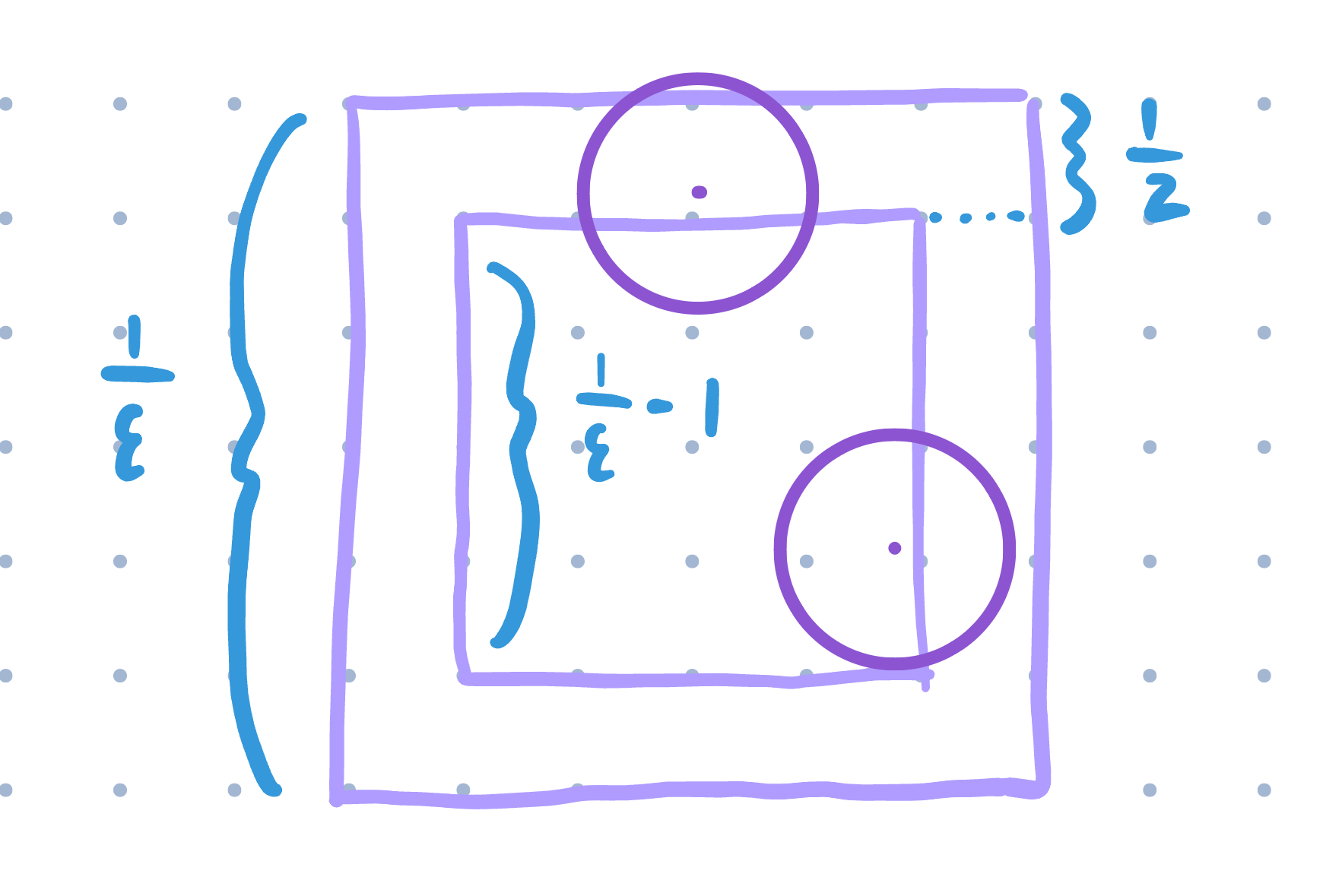
<p>If disks are within \(\dfrac{1}{2}\) of the grid line for a given grid square, then it will be removed. 
Our approximation only uses the ones that aren’t within \(\dfrac{1}{2}\) of the grid lines, or those that are within a \(\dfrac{1}{\epsilon} - \dfrac{1}{2} - \dfrac{1}{2}\) square inside the square. 
If we assume the disks are in a random position in the square, the probability is the area of the inner square minus the area of the outer square, which is the following</p>

\[\dfrac{\left(\dfrac{1}{\epsilon}-1\right)^2}{\dfrac{1}{\epsilon^2}} = \dfrac{\dfrac{(1-\epsilon)^2}{\epsilon^2}}{\dfrac{1}{\epsilon^2}} = (1-\epsilon)^2\]

<p>We are allowed to assume the disks are in a random position (relative to the grid lines) since we shift the grid by a random offset \(L\).
If we didn’t shift it, an adaptive offline adversary would be able to “set” the inputs to only disks that intersect the grid line, for example, which would return an independent set of size 0. 
Obviously, this isn’t a very good approximation!</p>

<p>So, this algorithm is a \((1-\epsilon)^2\) polynomial time approximation scheme for MISUDG!</p>

<h3 id="the-end">The End</h3>

<p>Thanks for reading! If you spot any mistakes (which are likely, this is unedited and kinda unchecked) then please feel free to reach out to me or fix them yourself on github issues. Or, if you have any insights, be sure to let me know!</p>]]></content><author><name></name></author><summary type="html"><![CDATA[In this post I’ll share a practice exercise I got from my CS 4540 class at Georgia Tech and my solution to it.]]></summary></entry><entry><title type="html">Voronoi Diagrams</title><link href="https://oriont.net/posts/delaunay-voronoi" rel="alternate" type="text/html" title="Voronoi Diagrams" /><published>2024-03-07T00:00:00+00:00</published><updated>2024-03-07T00:00:00+00:00</updated><id>https://oriont.net/posts/delaunay-voronoi</id><content type="html" xml:base="https://oriont.net/posts/delaunay-voronoi"><![CDATA[<h2 id="intro">Intro</h2>

<p>Recently, my research has involved going into Delaunay triangulations and Voronoi diagrams, here is what I’ve learned so far. If you find any errata please feel free to reach out to me via email on my contact page!</p>

<h2 id="definitions">Definitions</h2>

<p>Let \(P \subset \mathbb{R}^d\) be a set of points that we are interested in.</p>

<p>We define the Voronoi region \(V_S\) of a subset \(S \subset P\) of points as the intersection of halfspaces of each point in and out of the subset.</p>

\[V_S = \bigcap \limits_{\forall x \in S,\; y \in P \backslash S} H(x, y)\]

<p>Here, \(P \backslash S\) is the largest subset of \(S\) that doesn’t contain any item \(P\) contains. 
Also, \(H(x, y)\) is the halfspace on the side of \(x\). 
This is the region of \(\mathbb{R}^n\) such that each point it contains has \(S\) as its closest \(k=|S|\) neighbors.</p>

<p>We define the order-k Voronoi diagram \(\mathbb{V}_k (P)\) as the set of all such regions.</p>

\[\mathbb{V}_k (P) = \{V_S \mid S \subset P \wedge |S| = k\}\]

<p>Here, 
\(|S|\) 
is the cardinality of set S.</p>

<p>There are multiple definitions for the voronoi diagram, but this is my favorite so far because of it’s combinatorial nature; it lets us think of each region as corresponding to a subset of the points.</p>

<p>We let 
\(|\mathbb{V}_k (P)|\)
denote the number of regions the Voronoi diagram contains. This value is constrained by the amount of possible subsets of $P$, as per our definition.</p>

<p>This means we can impose the constraint 
\(|\mathbb{V}_k (P)| \leq {|P| \choose k}\)
.</p>

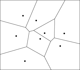
<p>Looking at a picture of an order-k 2-dimensional Voronoi diagram lets us see how many regions there are. 
Obviously in this case, there are less than \({|P| \choose k}\) regions. My research is interested in the upper and lower bounds on \(|\mathbb{V}_k (P)|\), along with conditions on \(P\) that allow us to make the bound tighter.</p>

<p><img src="/assets/images/voronoi.gif" alt="Voronoi" /></p>

<h3 id="another-definition">Another definition</h3>

<p>Voronoi regions can also be defined as follows:</p>

\[V_S = \{x \in \mathbb{R}^d \mid d(x, y) \leq d(x, z) \; \forall y \in S,\; z \in P \backslash S\}\]

<p>where \(d(x, y)\) is some distance metric between points \(x\) and \(y\). This definition emphasizes how the region contains \(S\) as its nearest neighbors.</p>

<h2 id="properties">Properties</h2>

<p>Now we delve into some cool properties of Voronoi diagrams.</p>

<ol>
  <li>
    <p>Each Voronoi region is a convex set.</p>

    <p>A convex set is a set \(S\) in which any combination of elements \(\alpha s_i + \beta s_j \in S\) where \(\alpha + \beta = 1\) and \(\alpha, \beta \in (0, 1)\).</p>

    <p>Notice in the picture how some regions can be infinite, or <strong>open</strong>.
 This doesn’t violate the convex set property. 
 A naive way to think about this is that each region is made out of purely convex corners.</p>

    <p>Maybe I’ll provide a proof for this in the future…</p>

    <p>This property allows us to use convex optimization techniques, which have been studied in depth, to optimize functions in Voronoi regions, which can be useful in machine learning applications, or in constructing diagrams as in <a href="https://dl.acm.org/doi/10.1145/100216.100259">Mulmuey 1990</a>.</p>

    <p>#### Plug!</p>

    <p>Side note: for my research I’m trying to figure out if the following conjecture made in the Mulmuley paper is true or not:</p>

    <blockquote>
      <p>\(\Omega(k^d n)\) is almost certainly a lower bound [of 
 \(|\mathbb{V}_k (P)|\)
 ] but the proof seems elusive.</p>
    </blockquote>

    <p>If you happen to have any information on this, please let me know!</p>
  </li>
  <li>
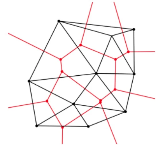
    <p>The graph dual of a 2-dimensional order-1 Voronoi diagram is the unique Delaunay Triangulation corresponding to \(P\).</p>

    <p><img src="/assets/images/voronoi_delaunay.webp" alt="Voronoi Delaunay" /></p>

    <p>In the future, I’ll probably make a post on Delaunay triangulations as well. Refer to the above picture for the graph dual of a Voronoi diagram. <br />
 (The voronoi diagram is in red, the Delaunay triangulation is in black)</p>

    <p>Each Voronoi region has a point in the Delaunay triangulation, and these points are connected if the regions share an edge.</p>

    <p>Higher dimensional Delaunay “mosaics” exist as well for higher dimensional and higher order Voronoi diagrams as well, but they haven’t studied as completely as 2-dimensional order-1 diagrams.</p>
  </li>
</ol>

<h2 id="some-applications">Some Applications</h2>

<p>There are tons of applications of Voronoi diagrams and Delaunay triangulations in fields like crystallography, but I am more interested in machine learning.</p>

<ol>
  <li>
    <p>Simple classifiers</p>

    <p>For classifiers such as \(k\)-Nearest Neighbors classifiers, Voronoi diagrams show which regions sample data can be located in to categorize as certain classes.</p>
  </li>
  <li>
    <p>HNSW</p>

    <p>The reason I got into this area of research was because as I was going through the HNSW paper, I noticed they make this bold assumption that slightly randomized small worlds graphs approximate Delaunay triangulations and don’t provide any backing behind it.</p>

    <p>Delaunay triangulation graphs have high navigability properties, ideal for graph search, which HNSW builds on in their paper. In practice, HNSW shows incredible results akin to logarithmic, as specified in the paper. But, the theoretical grounds haven’t been fully covered as far as I can tell.</p>
  </li>
</ol>

<h2 id="the-end">The End</h2>

<p>Thanks for reading! If you’re interested in what I’m doing, feel free to reach out and contact me!</p>]]></content><author><name></name></author><summary type="html"><![CDATA[Intro]]></summary></entry><entry><title type="html">Memory in LLMs</title><link href="https://oriont.net/posts/llm-memory" rel="alternate" type="text/html" title="Memory in LLMs" /><published>2023-06-17T00:00:00+00:00</published><updated>2023-06-17T00:00:00+00:00</updated><id>https://oriont.net/posts/llm-memory</id><content type="html" xml:base="https://oriont.net/posts/llm-memory"><![CDATA[<p>Large Language Models (LLMs) are very popular today, especially with new apps/libraries making them extremely easy to work with (i.e. <a href="https://python.langchain.com/docs/get_started/introduction.html">LangChain</a>). However, when I started working with them, I ran into a problem pretty quickly, namely that I wanted my ‘chatbot’ to be able to remember the current conversation. Without memory, LLMs can only respond to a single question at a time before forgetting all this ‘context’.</p>

<h2 id="the-problem-in-more-detail">The Problem in More Detail</h2>

<p>LLM APIs such as <a href="https://platform.openai.com/docs/models">OpenAI’s gpt models</a>, Facebook’s models including <a href="https://ai.facebook.com/blog/large-language-model-llama-meta-ai/">LLAMA</a>, <a href="https://huggingface.co/spaces/HuggingFaceH4/open_llm_leaderboard">huggingface’s transformer-based models</a> and any many other models are all stateless. This means that their model outputs will depend solely on the input you provide. The problem arises with the fact that most LLM applications are stateful. For example, chatbots (like ChatGPT) need to remember what was said earlier in the conversation to be able to respond on topic. However, there has been a lot of work done on <strong>memory</strong>, which are ways to transform these state<strong>less</strong> models into (pseudo) state<strong>ful</strong> models.</p>

<h2 id="memory-in-rnns">Memory in RNNs</h2>

<p>Modern language models are generally based on the transformer architecture, which came out in the groundbreaking <a href="https://arxiv.org/abs/1706.03762">Attention is All you need paper</a>. This paper essentially rendered recurrent neural networks (RNNs) worthless because of the strong attention improvement made possible by transformers. However, by switching to transformers, we abandon a very interesting property of RNNs; their own built-in memory.</p>

<p>RNNs use a <strong>previous state</strong> along with the current token as input, to predict the next token. The sequential nature of this model means training on GPUs, which are highly optimized for parallel computation, is much slower. (This is one of the reasons transformers are deemed ‘better’) But, the fact that the <strong>previous state</strong> is being used means it has its own <strong>built in memory</strong>. Theoretically, by encoding the previous context, whether that be a conversation, weather data, or stock prices, the RNN, a state machine technically, can make a prediction based on that. Note the impracticality of encoding any normal amount of data into a single vector (the conventional way for RNNs). This likely means much of the data is lost in the process, and only certain (hopefully important) properties are preserved. However, I like how this <strong>memory</strong> (state) is inherent in the model of an RNN.</p>

<p>Transformers are fundamentally different. Instead of sequentially calculating each token, an attention matrix is calculated and the output is calculated in one computation. This means that the memory must somehow be included in the input/attention matrix. Which brings us to the next section.</p>

<h2 id="memory-for-chatbots">Memory for Chatbots</h2>

<p>There are many ways to implement memory into chatbot LLMs, including</p>

<ol>
  <li>
    <p><a href="https://python.langchain.com/docs/modules/memory/how_to/buffer">Conversation Buffer Memory</a>
This kind of memory very simple. Each time you query the chatbot for a message, you basically just paste the entire previous conversation right before your next response and feed that into the LLM. The benefits of this include that it’s very simple and doesn’t get rid of any data. A big disadvantage of this method is that since LLM APIs usually have a token limit, the LLM won’t be able to respond after a long enough conversation. In other words, it’s not scalable.</p>
  </li>
  <li>
    <p><a href="https://python.langchain.com/docs/modules/memory/how_to/summary">Conversation Summary Memory</a>
Every message and response sent, a summary is created of the previous summary combined with the new message and response. Of course, the initial summary is nothing. This is called a “rolling summary” and is updated for each interaction. To make the summary, another LLM is used, whether it’s the same or a different one. An advantage of this is that while still being simple, it also allows for much better scaling: even if the conversation gets really long, the summary can just contain the key points and stay a certain length. However, the big disadvantage of this way is that it loses details.</p>
  </li>
  <li>
    <p><a href="https://python.langchain.com/docs/modules/memory/how_to/entity_summary_memory">Conversation Entity Memory</a>
An external state, such as a simple key value store is used to store summaries/definitions of what certain entities/objects/concepts are. Each prompt is analyzed to determine which definitions to include, and which to update, and the response uses these summaries as context. An advantage of this method is being able to see exactly which entities are being prioritized, and seeing if the state definitions are true to what the user intended. However, a disadvantage is that this method begins to complicate pipelines to language model calls.</p>
  </li>
  <li>
    <p><a href="https://python.langchain.com/docs/modules/memory/how_to/kg">Conversation Knowledge Graph Memory</a>
This method is similar to entity memory, but instead of using a key value store, a knowledge graph is used. Each interaction results in graph nodes being changed/created, and the knowledge graph is used as context for the next interaction. I don’t know much about knowledge graphs, so I’m interested in playing around with them in the future.</p>
  </li>
</ol>

<h2 id="other-memory">Other Memory</h2>

<ul>
  <li><a href="https://arxiv.org/pdf/2304.03442.pdf">Generative Agents Paper</a>. This paper proposes using architectures that reflect on observations for “high-level inferences”, store their reflections, and retrieve them for later usage. The components of their model are called the “memory stream”, “reflection”, and “planning”. To me, this seems like an attempt to model human behavior; as a human myself, I observe things in my memory stream, I reflect and think about them, and then I decide what to do with this new information.</li>
</ul>

<h2 id="closing-remarks">Closing Remarks</h2>

<p>The memory methods I discussed mostly only apply to chatbots, despite there being many more different applications than just chatbots. However, some of the methods can be transcribed to other applications pretty easily, which I may discuss in a later post.</p>

<p>This blog post was partially inspired by <a href="https://www.youtube.com/watch?v=3fge-zqZezw">Harrison Chase’s speech on Memory in LLM Applications at the Weights &amp; Biases Fully Connected Conference</a>, which I was fortunate enough to be able to attend.</p>

<p>Thanks for reading!</p>]]></content><author><name></name></author><category term="post" /><category term="ai" /><summary type="html"><![CDATA[Large Language Models (LLMs) are very popular today, especially with new apps/libraries making them extremely easy to work with (i.e. LangChain). However, when I started working with them, I ran into a problem pretty quickly, namely that I wanted my ‘chatbot’ to be able to remember the current conversation. Without memory, LLMs can only respond to a single question at a time before forgetting all this ‘context’. The Problem in More Detail LLM APIs such as OpenAI’s gpt models, Facebook’s models including LLAMA, huggingface’s transformer-based models and any many other models are all stateless. This means that their model outputs will depend solely on the input you provide. The problem arises with the fact that most LLM applications are stateful. For example, chatbots (like ChatGPT) need to remember what was said earlier in the conversation to be able to respond on topic. However, there has been a lot of work done on memory, which are ways to transform these stateless models into (pseudo) stateful models. Memory in RNNs Modern language models are generally based on the transformer architecture, which came out in the groundbreaking Attention is All you need paper. This paper essentially rendered recurrent neural networks (RNNs) worthless because of the strong attention improvement made possible by transformers. However, by switching to transformers, we abandon a very interesting property of RNNs; their own built-in memory. RNNs use a previous state along with the current token as input, to predict the next token. The sequential nature of this model means training on GPUs, which are highly optimized for parallel computation, is much slower. (This is one of the reasons transformers are deemed ‘better’) But, the fact that the previous state is being used means it has its own built in memory. Theoretically, by encoding the previous context, whether that be a conversation, weather data, or stock prices, the RNN, a state machine technically, can make a prediction based on that. Note the impracticality of encoding any normal amount of data into a single vector (the conventional way for RNNs). This likely means much of the data is lost in the process, and only certain (hopefully important) properties are preserved. However, I like how this memory (state) is inherent in the model of an RNN. Transformers are fundamentally different. Instead of sequentially calculating each token, an attention matrix is calculated and the output is calculated in one computation. This means that the memory must somehow be included in the input/attention matrix. Which brings us to the next section. Memory for Chatbots There are many ways to implement memory into chatbot LLMs, including Conversation Buffer Memory This kind of memory very simple. Each time you query the chatbot for a message, you basically just paste the entire previous conversation right before your next response and feed that into the LLM. The benefits of this include that it’s very simple and doesn’t get rid of any data. A big disadvantage of this method is that since LLM APIs usually have a token limit, the LLM won’t be able to respond after a long enough conversation. In other words, it’s not scalable. Conversation Summary Memory Every message and response sent, a summary is created of the previous summary combined with the new message and response. Of course, the initial summary is nothing. This is called a “rolling summary” and is updated for each interaction. To make the summary, another LLM is used, whether it’s the same or a different one. An advantage of this is that while still being simple, it also allows for much better scaling: even if the conversation gets really long, the summary can just contain the key points and stay a certain length. However, the big disadvantage of this way is that it loses details. Conversation Entity Memory An external state, such as a simple key value store is used to store summaries/definitions of what certain entities/objects/concepts are. Each prompt is analyzed to determine which definitions to include, and which to update, and the response uses these summaries as context. An advantage of this method is being able to see exactly which entities are being prioritized, and seeing if the state definitions are true to what the user intended. However, a disadvantage is that this method begins to complicate pipelines to language model calls. Conversation Knowledge Graph Memory This method is similar to entity memory, but instead of using a key value store, a knowledge graph is used. Each interaction results in graph nodes being changed/created, and the knowledge graph is used as context for the next interaction. I don’t know much about knowledge graphs, so I’m interested in playing around with them in the future. Other Memory Generative Agents Paper. This paper proposes using architectures that reflect on observations for “high-level inferences”, store their reflections, and retrieve them for later usage. The components of their model are called the “memory stream”, “reflection”, and “planning”. To me, this seems like an attempt to model human behavior; as a human myself, I observe things in my memory stream, I reflect and think about them, and then I decide what to do with this new information. Closing Remarks The memory methods I discussed mostly only apply to chatbots, despite there being many more different applications than just chatbots. However, some of the methods can be transcribed to other applications pretty easily, which I may discuss in a later post. This blog post was partially inspired by Harrison Chase’s speech on Memory in LLM Applications at the Weights &amp; Biases Fully Connected Conference, which I was fortunate enough to be able to attend. Thanks for reading!]]></summary></entry><entry><title type="html">Introduction to Blockchains</title><link href="https://oriont.net/posts/blockchain-intro" rel="alternate" type="text/html" title="Introduction to Blockchains" /><published>2022-02-05T00:00:00+00:00</published><updated>2022-02-05T00:00:00+00:00</updated><id>https://oriont.net/posts/blockchain-intro</id><content type="html" xml:base="https://oriont.net/posts/blockchain-intro"><![CDATA[<h1 id="introduction">Introduction</h1>

<p>Web 1.0 was based on static html pages on websites (kind of like this blog).
Web 2.0 is based on more dynamic structures, allowing for the creation of new pages and manipulation of data on the website.
Web 3.0 is based on decentralization–what better tool to advance this technology than blockchain?</p>

<p>For example, say you store all your photos on your computer.
If someone breaks into your house and steals your computer, then your photos are gone.
Or, if your computer catches on fire somehow, your photos are gone.
Or, if you accidentally delete your photos permanently, then your photos are gone.
The point is that there are many ways for a single system to fail, and if your application is centralized, failing will have dire consequences.</p>

<p>With a decentralized system, your photos would be stored across hundreds (or thousands!) of computers.
This way, if something happened to your computer, your photos wouldn’t be gone forever.
You could just ask someone else in the network (who has a working computer) for them!</p>

<p>Of course, this wouldn’t work if every single computer in the network was broken; there would be no one to ask.
However, such a catastrophe is very unlikely to happen; decentralized networks incentivize network “nodes” to stay online.
This incentive depends on the network you are using: bitcoin, ethereum, solana, arweave, etc.</p>

<h1 id="how-do-you-make-a-decentralized-network">How do you make a decentralized network?</h1>

<p>Decentralized networks work because they can synchronize one state across many nodes.
The “state” can be thought of as all the data that is stored on the blockchain at a point in time.
So, how can we synchronize state?</p>

<p>Let’s use an example:
Fred and his friends want to make a decentralized network.
They decide to manually do all operations.
Fred decides to put some text on the network: “bananafdjskal;”
Obviously, there is a typo–Fred meant to type “banana”.
Before he noticed his typo, he told all his friends to put “bananafdjskal;” onto their network.
Now, the network state looks like this:</p>

<div class="language-plaintext highlighter-rouge"><div class="highlight"><pre class="highlight"><code>Fred's essay: "bananafdjskal;"
</code></pre></div></div>

<p>Fred decides to fix his typo.
He tells all his friends to replace his word with “banana”.
Now, the state looks like this:</p>

<div class="language-plaintext highlighter-rouge"><div class="highlight"><pre class="highlight"><code>Fred's essay: "banana"
</code></pre></div></div>

<p>Fred and his friends have just successfully made a decentralized network!
But, we haven’t tested any of the problems…</p>

<h1 id="common-problems">Common Problems</h1>

<p>Imagine Caroline tries to edit Fred’s essay.
We don’t want Caroline to be able to edit Fred’s essay, because Fred is the one writing it, not Caroline!
So, in order for a change to be made, we have to confirm the person making the change is the person who owns the essay.
A common way to do this is to use a signature.
When you buy something at a store with a credit card, you have to put in a pin or sign your name.
Whenever Fred wants</p>

<p>UNFINISHED!</p>]]></content><author><name></name></author><category term="post" /><category term="blockchain" /><summary type="html"><![CDATA[Introduction]]></summary></entry><entry><title type="html">Intro to Data Augmentation</title><link href="https://oriont.net/posts/data-augmentation" rel="alternate" type="text/html" title="Intro to Data Augmentation" /><published>2021-11-30T00:00:00+00:00</published><updated>2021-11-30T00:00:00+00:00</updated><id>https://oriont.net/posts/data-augmentation</id><content type="html" xml:base="https://oriont.net/posts/data-augmentation"><![CDATA[<p>Datasets are the heart of any machine learning model.
We use them to fine tune the model’s parameters in order to make better predictions.</p>

<p>A big factor in the accuracy of the predictions is the quality of data provided.
We may use different models and training algorithms to improve the accuracy of our model, but none of that matters if we have bad data.
For example, imagine we want to train a model to recognize if a picture contains text.
Our dataset could consist of thousands of images of many different books as the text images, and paintings, clothing, and houses as the non-text images.
When we train the model, it should be able to tell apart books from houses. Great!</p>

<p>However, what if we show the model a car with a bumper sticker?
The model was trained on only different books, so it probably won’t recognize the text unless it is encapsulated in a nice white rectangle. (page of a book)
It could go the other way as well: the model would likely predict that an image contains text, if that image is a page of a book with scribbles on it instead of text.</p>

<p>Now, consider we had a much more diverse dataset, full of books, signs, papers, bumper stickers, receipts, and text messages classified as text, and paintings, houses, cars, mountains, forests, and animals classified as no-text.
A model trained off of this new dataset would probably be able to detect if an image has text with much more accuracy than the last model.
Since there is more variety in our training data, the model won’t overfit to a certain type of data and will be more likely to classify abstract cases correctly.
So, it would probably predict that a computer screen with this post has text, and it would also likely predict that a scene from a video game doesn’t.</p>

<h1 id="small-datasets">Small Datasets</h1>

<p>Collecting data can be super annoying.
Sometimes, entering all the (potentially thousands of) features takes egregious amounts of time. (Handwritten surveys, for example.)
Other times, data points are hard to come by. (Light bent by a black hole, for example.)</p>

<p>When I refer to small datasets, I’ll be talking about datasets with less than 1000 entries.
Realistically however, small datasets by today’s standards can contain tens or hundreds of thousands of entries.</p>

<p>It’s possible to train models on small datasets.
With smart model engineering, careful hyperparameter tuning, and correctly-sized validation/testing sets, very good models can be trained on minimal data.</p>

<p>However, it’s generally safer (and much easier) to train models on large datasets.
This is because the model parameters can be adjusted more according to the dataset, but since there are more values, it won’t be overfitted to a few values.</p>

<h1 id="expanding-your-datasets">Expanding Your Datasets</h1>

<p>What do you do if you have a limited amount of data, but want a larger dataset for training your model?
<a href="https://en.wikipedia.org/wiki/Data_augmentation">Data augmentation</a> can be a great solution.</p>

<p>Data augmentation is the act of expanding an existing dataset by creating altered copies of the original data.
Altered copies can be created in infinite ways: simple transformations are most commonly used.
For any dataset, we can add small amounts of noise to each value in the dataset.
This should keep the data representative of what it was before, since the noise is small.
However, adding noise that is too large can harm the data, which makes it useless.
Access caution!</p>

<p>For images specifically, we can get a little creative with data augmentation.
Actions such as cropping the image, rotating the image, and flipping the image are easy to implement and effective ways to augment your data.
Less common ways include blurring, color swapping, inverting, and dialating the image.</p>

<p>If the image is made smaller but kept as the same size in pixels, it will have a blank background.
This can be harmful to models, since the drastic change in variety of color and non-zero values will be very easy for the model to pick up on, which can lead to the model training incorrectly.
So, the image can be flipped and repeated on each edge as a slight remedy.
Notice, however, that this can still cause strange outputs in your model.</p>

<h1 id="overfitting">Overfitting</h1>

<p>Not all datasets are small.
In the case of a large dataset and a very complex model, data augmentation can still help!</p>

<p>By adding slightly altered versions of the image, we are essentially performing a <a href="https://en.wikipedia.org/wiki/Regularization_(mathematics)">regularization technique</a>.
Regularization is the act of reducing overfitting; in this case, the added data will increase the chances of the model picking up more general patterns, instead of learning the exact patterns from our dataset, which will result in a better performing model.</p>

<p>The problem of overfitting (relevant to data augmentation) will only arise when your model is sufficiently complex (a very deep neural network, perhaps?) compared to the dataset, despite it being medium to large in size.
So, it’s best to use your own judgement to use it or not in such cases.
Or, maybe you could train a model with data augmentation and another without it, and choose whichever one performs better as the final model.</p>

<h1 id="tensorflow">TensorFlow</h1>

<p>Luckily, data augmentation tools are provided with tensorflow, which is a commonly used library in machine learning for models and data modification.
They have a great guide on their documentation, <a href="https://www.tensorflow.org/tutorials/images/data_augmentation">which can be found here.</a></p>

<p>Data augmentation can be performed in pretty much any library.
Another common python library is numpy, <a href="https://medium.com/@schatty/image-augmentation-in-numpy-the-spell-is-simple-but-quite-unbreakable-e1af57bb50fd">which also can be used for data augmentation.</a></p>]]></content><author><name></name></author><category term="post" /><category term="machine-learning" /><summary type="html"><![CDATA[Datasets are the heart of any machine learning model. We use them to fine tune the model’s parameters in order to make better predictions.]]></summary></entry><entry><title type="html">Quick Setup For TensorFlow on Windows 10</title><link href="https://oriont.net/posts/tensorflow-gpu-setup" rel="alternate" type="text/html" title="Quick Setup For TensorFlow on Windows 10" /><published>2021-08-08T00:00:00+00:00</published><updated>2021-08-08T00:00:00+00:00</updated><id>https://oriont.net/posts/tensorflow-gpu-setup</id><content type="html" xml:base="https://oriont.net/posts/tensorflow-gpu-setup"><![CDATA[<p>I was working with tensorflow to make my GAN recently, but I noticed a couple things.
First, each epoch in training would take around 5 minutes, which is extremely slow.
For my goal of 100 epochs, it would take 500 minutes, which turns out to be over 8 hours.
Obviously, this is NOT ideal.</p>

<p>Then, I noticed another thing, and that was the small “missing dll” errors in my console!
As it turns out, you can use your GPU(s) to highly accelerate machine learning operations, because of all the matrix math optimizations offered by GPUs.
However, setting up tensorflow to utilize all your GPUs was, to put it lightly, a massive pain.
In this post, I’ll go over how to quickly install tensorflow and the correct cuda programs.</p>

<h1 id="hardware">Hardware</h1>

<p>This will only work if you currently have a CUDA-enabled GPU installed.
So pretty much any graphics card from NVidia should work.
For me, I have dual SLI GTX 970s.</p>

<p>I have a Windows 10 PC. That means that if you have a mac or linux PC, you should follow a different tutorial.</p>

<h1 id="todo-list">TODO List</h1>

<p>(Prerequisites)</p>

<ol>
  <li><a href="https://python.org">Install Python 3.9.x</a></li>
  <li><a href="https://pip.pypa.io/en/stable/installation/">Install PyPI</a></li>
  <li><a href="https://support.microsoft.com/en-us/topic/the-latest-supported-visual-c-downloads-2647da03-1eea-4433-9aff-95f26a218cc0">Install visual C++ redistributable</a></li>
</ol>

<p>(TODO) 3. Install TensorFlow 4. Install NVidia Drivers 5. Install CUDA Toolkit 6. Install CUDNN</p>

<h1 id="install-tensorflow">Install TensorFlow</h1>

<p>In a command prompt:</p>

<div class="language-plaintext highlighter-rouge"><div class="highlight"><pre class="highlight"><code>pip install --upgrade pip
pip install tensorflow
</code></pre></div></div>

<p>This just upgrades <code class="language-plaintext highlighter-rouge">pip</code> and installs the <code class="language-plaintext highlighter-rouge">tensorflow</code> package.
If you want to install a specific version, use the following syntax:</p>

<div class="language-plaintext highlighter-rouge"><div class="highlight"><pre class="highlight"><code>pip install tensorflow==2.6.0rc2
</code></pre></div></div>

<p>(If you want a list of versions, just use an unknown version and <code class="language-plaintext highlighter-rouge">pip</code> should tell you.)</p>

<div class="language-plaintext highlighter-rouge"><div class="highlight"><pre class="highlight"><code>pip i tensorflow==chicken
</code></pre></div></div>

<p>Since TensorFlow and CUDA are so picky about their versions, here is the version I used when I got it working: <em>2.6.0rc2</em>.</p>

<h1 id="install-nvidia-drivers">Install NVidia Drivers</h1>

<p>I recommend downloading GeForce experience, so you can keep your drivers updated automatically.
<a href="https://www.nvidia.com/en-us/geforce/geforce-experience/">You can find it here.</a></p>

<p><a href="https://www.nvidia.com/download/index.aspx?lang=en-us">Or, you can download drivers for a specific GPU here.</a></p>

<h1 id="install-cuda-toolkit">Install CUDA Toolkit</h1>

<p><a href="https://developer.nvidia.com/cuda-toolkit-archive">You can find a list of all the different versions of the CUDA toolkit here.</a></p>

<p>You’re probably wondering which version to install.
For my build, I installed <em>CUDA Toolkit 11.2.2</em>.</p>

<p>If tensorflow adds support for more recent versions of the CUDA Toolkit, you can try installing them for increased performance or new features.</p>

<p>Once you run the installer, you should have some new files in the following directory: <code class="language-plaintext highlighter-rouge">C:\Program Files\NVIDIA GPU Computing Toolkit\CUDA\v11.2</code>.</p>

<p>Before, if you ran a tensorflow project, you may have received an error similar to the following:</p>

<div class="language-plaintext highlighter-rouge"><div class="highlight"><pre class="highlight"><code>2021-08-08 17:12:44.906857: W tensorflow/stream_executor/platform/default/dso_loader.cc:64] Could not load dynamic library 'cudart64_110.dll'; dlerror: cudart64_110.dll not found
2021-08-08 17:12:44.906995: I tensorflow/stream_executor/cuda/cudart_stub.cc:29] Ignore above cudart dlerror if you do not have a GPU set up on your machine.
2021-08-08 17:12:46.625071: W tensorflow/stream_executor/platform/default/dso_loader.cc:64] Could not load dynamic library 'cudart64_110.dll'; dlerror: cudart64_110.dll not found
2021-08-08 17:12:46.626074: W tensorflow/stream_executor/platform/default/dso_loader.cc:64] Could not load dynamic library 'cublas64_11.dll'; dlerror: cublas64_11.dll not found
2021-08-08 17:12:46.627073: W tensorflow/stream_executor/platform/default/dso_loader.cc:64] Could not load dynamic library 'cublasLt64_11.dll'; dlerror: cublasLt64_11.dll not found
2021-08-08 17:12:46.628006: W tensorflow/stream_executor/platform/default/dso_loader.cc:64] Could not load dynamic library 'cufft64_10.dll'; dlerror: cufft64_10.dll not found
2021-08-08 17:12:46.628980: W tensorflow/stream_executor/platform/default/dso_loader.cc:64] Could not load dynamic library 'curand64_10.dll'; dlerror: curand64_10.dll not found
2021-08-08 17:12:46.629958: W tensorflow/stream_executor/platform/default/dso_loader.cc:64] Could not load dynamic library 'cusolver64_11.dll'; dlerror: cusolver64_11.dll not found
2021-08-08 17:12:46.631054: W tensorflow/stream_executor/platform/default/dso_loader.cc:64] Could not load dynamic library 'cusparse64_11.dll'; dlerror: cusparse64_11.dll not found
2021-08-08 17:12:46.632484: W tensorflow/core/common_runtime/gpu/gpu_device.cc:1835] Cannot dlopen some GPU libraries. Please make sure the missing libraries mentioned above are installed properly if you would like to use GPU. Follow the guide at https://www.tensorflow.org/install/gpu for how to download and setup the required libraries for your platform.
Skipping registering GPU devices...
</code></pre></div></div>

<p>This is because your computer can’t find the files listed in the error message.
But notice in the <code class="language-plaintext highlighter-rouge">bin</code> folder of the CUDA toolkit that we just installed, you can find all of these files.
This means, we need to add this folder to the path!</p>

<p>So, open the system environment variables by going to the start menu and searching “environment variables”.
Then, find the <code class="language-plaintext highlighter-rouge">Path</code> variable, select it, and click “edit”.
From there, you can click “New” to add a new directory to the path, and the directory you want to add is the directory containing all the missing libraries, aka <code class="language-plaintext highlighter-rouge">C:\Program Files\NVIDIA GPU Computing Toolkit\CUDA\v11.2\bin</code></p>

<p>Then, close out of the environment variables page, <em>making sure to apply your changes</em>.
Lastly, <em>RESTART all your currently open terminals. This is because the changes will not take place unless the terminal was created after you added the new path directory.</em></p>

<h1 id="install-cudnn">Install CUDNN</h1>

<p>Now, you may get an error similar to this:</p>

<div class="language-plaintext highlighter-rouge"><div class="highlight"><pre class="highlight"><code>2021-08-08 17:20:10.558894: W tensorflow/stream_executor/platform/default/dso_loader.cc:64] Could not load dynamic library 'cudnn64_8.dll'; dlerror: cudnn64_8.dll not found
2021-08-08 17:20:10.559029: W tensorflow/core/common_runtime/gpu/gpu_device.cc:1835] Cannot dlopen some GPU libraries. Please make sure the missing libraries mentioned above are installed properly if you would like to use GPU. Follow the guide at https://www.tensorflow.org/install/gpu for how to download and setup the required libraries for your platform.
Skipping registering GPU devices..
</code></pre></div></div>

<p>Now, it’s only missing one cuda dll, an it’s from CUDNN.
<a href="https://developer.nvidia.com/rdp/cudnn-download">You can find the most recent versions of CUDNN at this link.</a></p>

<p>NOTE: The site will prompt you to create an NVidia account and get a “Developer Program Membership”.
Don’t worry, this is super easy.</p>

<ol>
  <li>Create an account. (Or log in with google, or something)</li>
  <li>Verify your email</li>
  <li>Fill out your profile information. <em>Make sure to click the checkbox stating “Join the NVIDIA Developer Program to access downloads (like cuDNN), how-to videos, and more.”</em></li>
</ol>

<p>Now, you can go to the downloads page and download cuDNN.
The version that I got (which worked) is <em>v8.2.2 for CUDA 11.4</em>.
I know, I didn’t get CUDA Toolkit 11.4 (I got 11.2.2).
But, it still ended up working anyway!
If you want to match versions, please, feel free.</p>

<p>Once you downloaded the folder and extracted it into a new folder, place that folder somewhere it’ll be safe.
I just put it next to the CUDA toolkit, so my directory structure looked like this:</p>

<div class="language-plaintext highlighter-rouge"><div class="highlight"><pre class="highlight"><code>...
NVIDIA GPU Computing Toolkit
| - CUDA
  | - v11.2
  | | - bin/
  | ...
  | - cudnn-11.4-windows-x64-v8.2.2.26
    | - cuda
      | - bin/
      | - include/
      | - lib/
      | - NVIDIA_SLA_cuDNN_Support.txt
</code></pre></div></div>

<p>And, of course, we need to add this directory to the path environment variable.
Open up the environment variables, and add the <code class="language-plaintext highlighter-rouge">bin</code> directory to the path.</p>

<p>For me, it was the following:
<code class="language-plaintext highlighter-rouge">C:\Program Files\NVIDIA GPU Computing Toolkit\CUDA\cudnn-11.4-windows-x64-v8.2.2.26\cuda\bin</code></p>

<p>Now, since the <code class="language-plaintext highlighter-rouge">cudnn64_8.dll</code> file is in the path, we should be done with annoying errors!</p>

<h1 id="things-to-try-out">Things to try out</h1>

<p>An interesting project that I just did recently was training a GAN on the MNIST dataset.
<a href="https://machinelearningmastery.com/how-to-develop-a-generative-adversarial-network-for-an-mnist-handwritten-digits-from-scratch-in-keras/">Here is an amazing tutorial written by Jason Brownlee</a> which I highly recommend.</p>

<p>Fixing these GPU CUDA errors allowed python to fully utilize all the available computing resources I have.
This significantly cut down training times.
Previously, each epoch took about 5 minutes to train, whereas with the GPU acceleration, it only takes about 30 seconds.
I was able to train 100 epochs in less than an hour, thanks to these CUDA libraries!</p>

<p>If you want to play around with the model that I trained, <a href="https://github.com/eoriont/gan_mnist_playground_boilerplate">here is a github repository for it</a>.
Just clone the repository, and run the python file.
The model is stored in the <code class="language-plaintext highlighter-rouge">.h5</code> file.</p>

<p>I added some sliders so you can easily change the latent vector and see the live output.
Unfortunately, matplotlib has awful UI documentation, so about 70 of the sliders are off of the page.
Maybe someone can clean it up! (Just make a pull request)</p>]]></content><author><name></name></author><category term="post" /><category term="machine-learning" /><summary type="html"><![CDATA[I was working with tensorflow to make my GAN recently, but I noticed a couple things. First, each epoch in training would take around 5 minutes, which is extremely slow. For my goal of 100 epochs, it would take 500 minutes, which turns out to be over 8 hours. Obviously, this is NOT ideal.]]></summary></entry><entry><title type="html">Basic Introduction to Generative Adversarial Networks (GANs)</title><link href="https://oriont.net/posts/gan-intro" rel="alternate" type="text/html" title="Basic Introduction to Generative Adversarial Networks (GANs)" /><published>2021-08-01T00:00:00+00:00</published><updated>2021-08-01T00:00:00+00:00</updated><id>https://oriont.net/posts/gan-intro</id><content type="html" xml:base="https://oriont.net/posts/gan-intro"><![CDATA[<p>What is a neural network? You may have heard of neural networks before, and you may know that they mimic brains.
Many people’s knowledge on neural networks falters after that.
However, I’m here to provide a basic overview of what they are, and how they work.</p>

<p>A Neural Network, (or NN for short) is a model of how a brain could theoretically work.
I say model, because NNs are just complex structures made out of a bunch of tiny little parts.
In a real brain, these parts would be the neurons, and scientists have decided to name it the same thing in our model.
A NN is just a bunch of neurons connected to eachother.</p>

<p>Now, being modeled on the computer and restrained by the digital nature of silicon logic, it would take a lot of computation to simulate the exact voltages being pulsed through each neuron.
So, scientists have simplified it down to a bunch of linear equations, generally represented by vectors and matrices, carried out through dot products.</p>

<p>Why are we able to make approximations of neurons using linear algebra? Well, consider the structure of neurons in a real, human brain.</p>

<!-- Image of neurons in a human brain -->

<p><img src="/assets/images/ganintro_neurons.jpg" alt="Neurons" /></p>

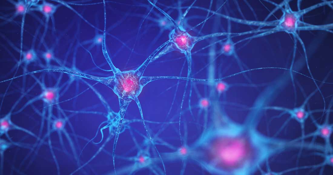
<p>Here, you can see how each neuron is connected to many other neurons, with varying connection “intensities”.
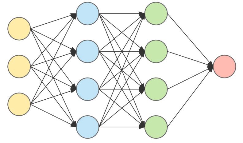
We can make our own model with similar properties, which can be visualized as the following.</p>

<!-- Image of neurons in a neural network -->

<p><img src="/assets/images/ganintro_neuralnetwork.jpg" alt="Neural Network" /></p>

<p>Notice the similar properties here.</p>

<ul>
  <li>Each neuron is connected to a number of other neurons.</li>
  <li>Each connection has a certain “intensity” or “weight”. (Can also be thought of as length)</li>
</ul>

<p>Also, notice some other properties.</p>

<ul>
  <li>Information/voltages/signals from each neuron only flows from left to right.</li>
  <li>There are input neurons. (Yellow)</li>
  <li>There are output neurons. (Red)</li>
  <li>The neurons in vertical columns can be grouped together and called “layers”, representing each “step” of getting an output.</li>
</ul>

<p>In a normal human brain with relatively unstructured neurons, we wouldn’t know where the network starts or ends!
However, modeling a network like this makes it much easier to find definite inputs and outputs, much less calculate outputs from certain inputs.
So, how can we calculate some outputs?
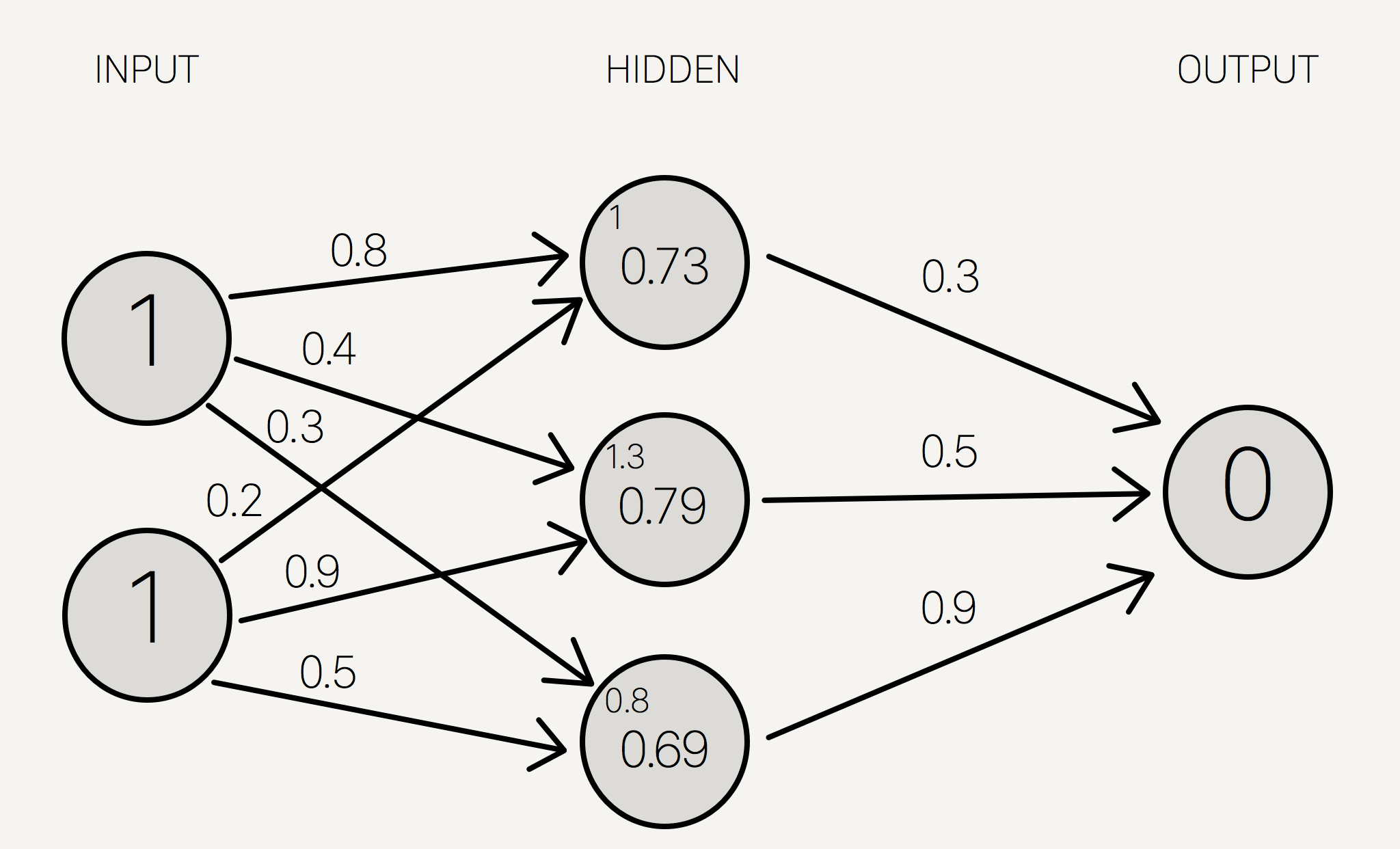
First, take some inputs, as a vector to represent each voltage level in the input layer.
Each connection/edge has a weight/intensity, so how can we represent the voltage encountering such resistance?
We can multiply the voltage by the edge weight.
This effectively represents the lessened/heightened voltage due to the connection strength.</p>

<p>Once we get all the voltages at the end of each connection, we need a way to combine them as input to the next node.
The easiest way to do that is just to get the arithmetic sum.
Now, we have the voltages of the first layer. Hooray!
In order to keep going, we repeat the process.</p>

<ol>
  <li>Multiply the input values by the edge weights.</li>
  <li>Add them up, and set the sum as the inputs to the next neuron.</li>
</ol>

<p>It’s that simple!
One who is familiar with linear algebra may recognize the act of adding a bunch of products.
That’s right; we can do this all with matrices, dot products, and matrix multiplication!
We have a vector of all the neuron inputs.
The weights corresponding to each output neuron can be put into a matrix, where every row corresponds to a different input neuron, and every column corresponds to a different output neuron.
Multiplying these two matrices will multiply each input value with each edge weight, sum them up nicely, and store it in a vector.
Linear algebra basically just served us neural networks on a silver platter!</p>

<h2 id="training-a-neural-network">Training a Neural Network</h2>

<p>This topic is much more complex, and could be put in its own blog post.
However, to get the gist of it:</p>

<p>We first have to have a bunch of data to train the network with.
That could be the color values of each pixel in an image, amounts of ingredients in certain cookies, survival statistics on the Titanic incident, etc.
We start out with a neural network with a bunch of random edge weights.
When we give it some inputs and calculate the output, the neural network will give us some weird random answer, due to all the random numbers in the weights.
In order for the network to give us sensible answers, we need to adjust each edge weight until the outputs become reasonable.
We can’t do this manually, though.</p>

<!-- Image of neural networks with weights -->

<p><img src="/assets/images/ganintro_nnweights.png" alt="Neural Network with Weights" /></p>

<p>So, we have a predicted output (from the neural network) and an actual output, from our dataset.
Given a theoretical value and an actual value, it’s trivial to calculate the percent error.
Obviously, we will want to minimize this error, because we want the neural network to give answers that represent real answers.</p>

<!-- Image of neural networks with squared errors -->

<p><img src="/assets/images/ganintro_nnerrors.jpg" alt="Neural Network with Errors" /></p>

<p>We adjust the weights of each neuron.
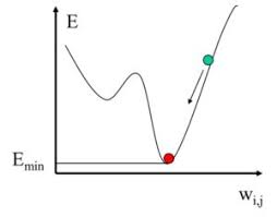
Our goal is to adjust each weight by minimizing the error of the entire network.
This can be done by adjusting each weight individually by a small amount and calculating the error for each adjustment.
Then, using basic calculus, we can use a central difference approximation to approximate the derivative of the error with respect to that edge.
From there, we can just adjust the weight to minimize the squared error, using the derivative approximation.</p>

<p>Then, we just do that for each edge, et voila!
We are left with a network that has slightly less error than before.</p>

<h1 id="what-is-deep-learning">What is Deep Learning?</h1>

<p>‘Deep Learning’ is a term that is often thrown around for many different machine learning models.
A combination of its denotation and some theory behind neural networks will be sufficient to understand its meaning.</p>

<p>Each layer in a neural network is a way for our model to recognize different patterns.
The first layer would be able to recognize simple patterns.
For example, it could recognize if two inputs were on at the same time, and output that.
This could be like an AND gate.
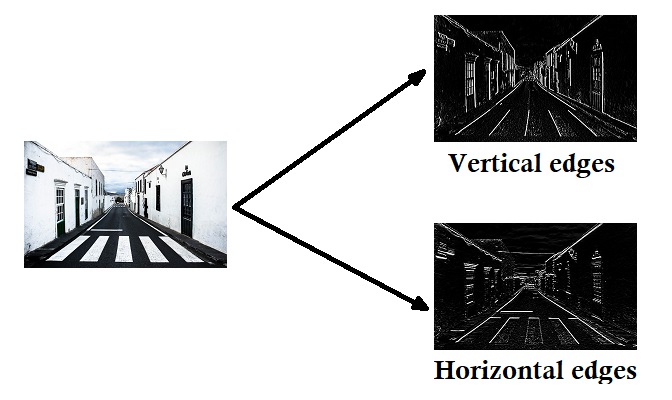
If we were using images, one node in the first layer may detect a vertical edge with black on the left side.
It could also detect vertical edges with black on the right side, horizontal edges, edges with different colors, and even dots or circles.</p>

<!-- Image of edge detection -->

<p><img src="/assets/images/ganintro_edgedetection.jpg" alt="Edge Detection" /></p>

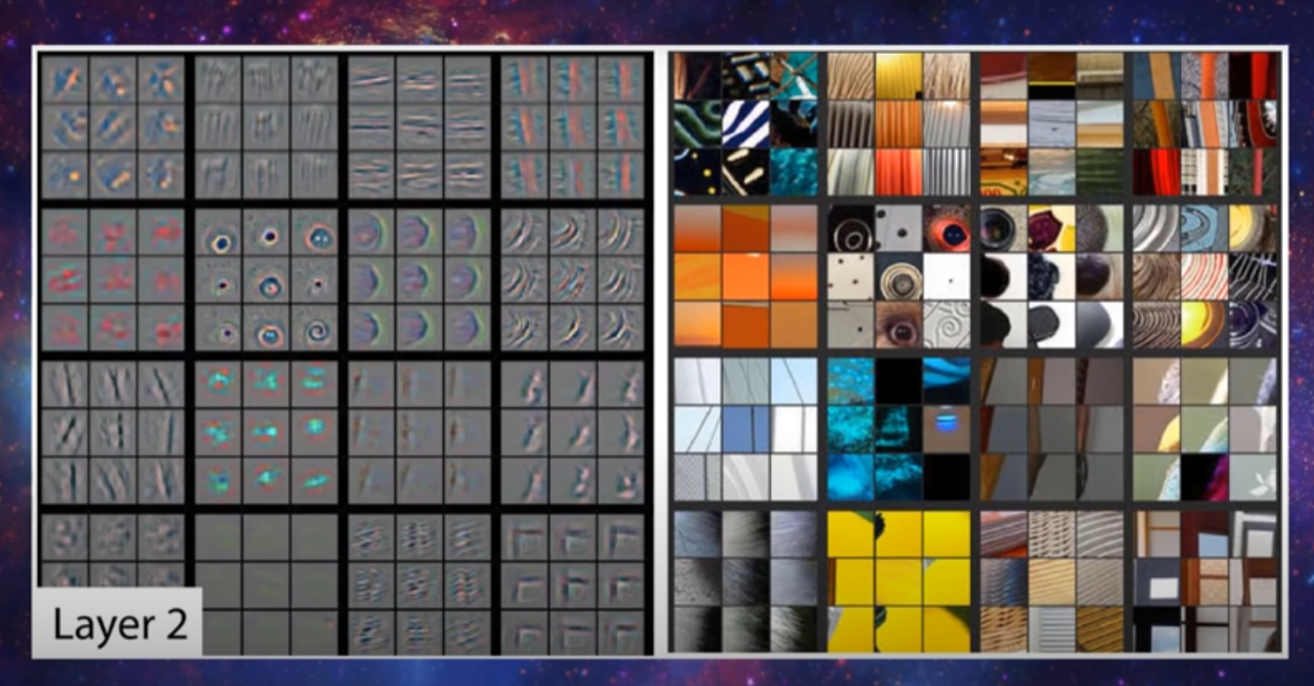
<p>Moving on to the second layer, we can use the simple patterns in the first layer to detect slightly more complex patterns.
For example, the network could combine multiple edges to detect a corner.
It could also detect parallel edges, which would signify a line.
Using extra edges and dots, it could detect a larger circle.</p>

<!-- Image of more complex pattern detection -->

<p><img src="/assets/images/ganintro_complexpattern.png" alt="Complex Patterns" /></p>

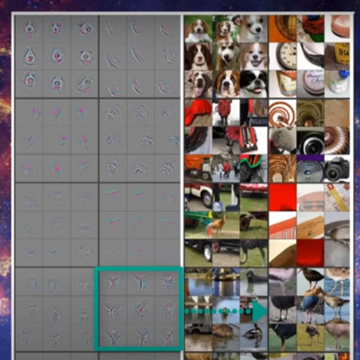
<p>For the third layer, the network could detect more complex patterns, like an actual eye or mouth.
Then, the fourth layer could detect a whole face, and the fifth layer may be able to detect a whole person.</p>

<!-- Image of even more complex pattern detection -->

<p><img src="/assets/images/ganintro_complexpattern2.png" alt="More Complex Patterns" /></p>

<p>As you can see, the more layers a neural network has, the more complex patterns it can actually detect.
When a network has the property of having a lot of layers, it is able to make more complex and deep connections within the dataset that it is given.
Hence, deep learning.</p>

<p>In basic terms, deep learning just means the network has many layers, or capacity for complexity.</p>

<p>The network I just described is definitely possible, but there are a few things one should note.
The first thing is that you don’t actually define each node as being able to “recognize” certain patterns, like edges, corners, eyes, or people.
When you train the network, it <em>alters itself</em> to be able to detect certain patterns.
Obviously, the stated patterns are possibilities.
However, trained neural networks tend to be convoluded.
They usually develop their own patterns, like maybe if a couple strange colors are near eachother.</p>

<p>Using traditional methods of training, as explained above, it wouldn’t be possible to set the patterns that the network understands.
Instead, it chooses its own patterns, through it adjusting its edge weights by minimizing error.</p>

<p>The second thing we should note, is that I described a convolutional neural network.
Normal neural networks would have to be able to recognize a pattern on <em>every single combination of pixels</em>, which would take a lot more neurons per layer.
However, convolutional neural networks are able to use a cool trick to recognize patterns anywhere.</p>

<h1 id="convolutional-neural-networks-cnns">Convolutional Neural Networks (CNNs)</h1>

<p>The main difference between a convolutional neural network and a normal neural network is the convolutional layers.
This is where a <em>filter</em> is created, and convolved around the image.</p>

<p>A filter can be thought of as transparent tracing paper.
It contains pixel values, like an image, but it’s main purpose isn’t to be observed, rather, to be compared.</p>

<!-- Image of transparent tracing paper -->

<p><img src="/assets/images/ganintro_transparentpaper.jpg" alt="Transparent Tracing Paper" /></p>

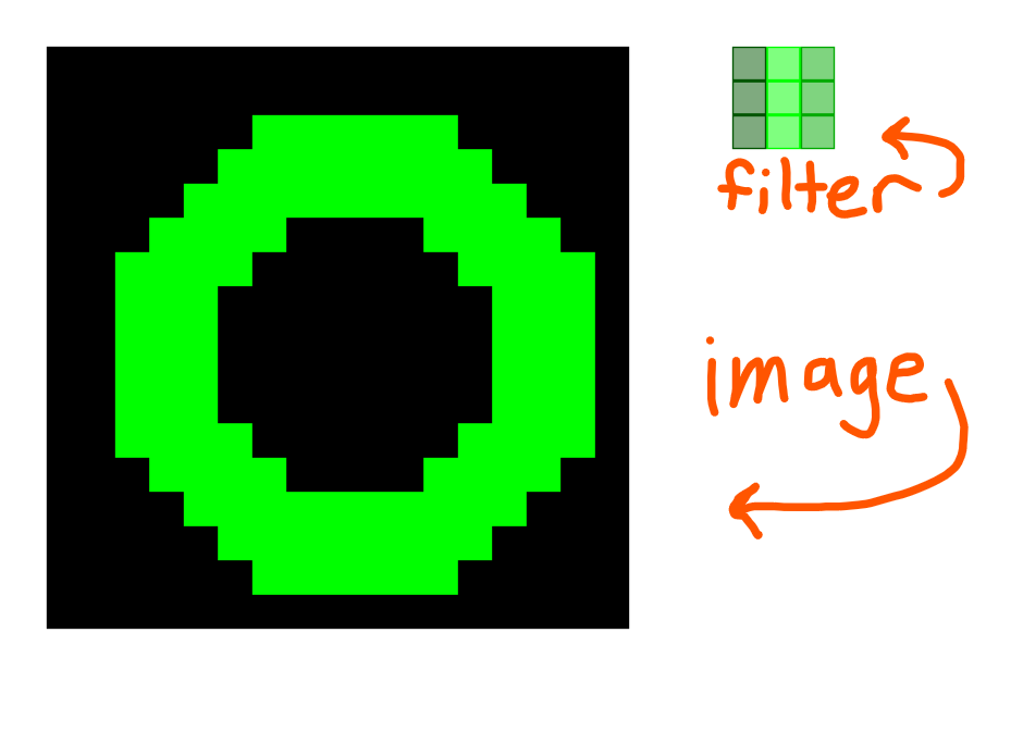
<p>Imagine our input is the rgb values for each pixel in an image.</p>

<!-- Image of filter -->

<p><img src="/assets/images/ganintro_convfilter.png" alt="Filter" /></p>

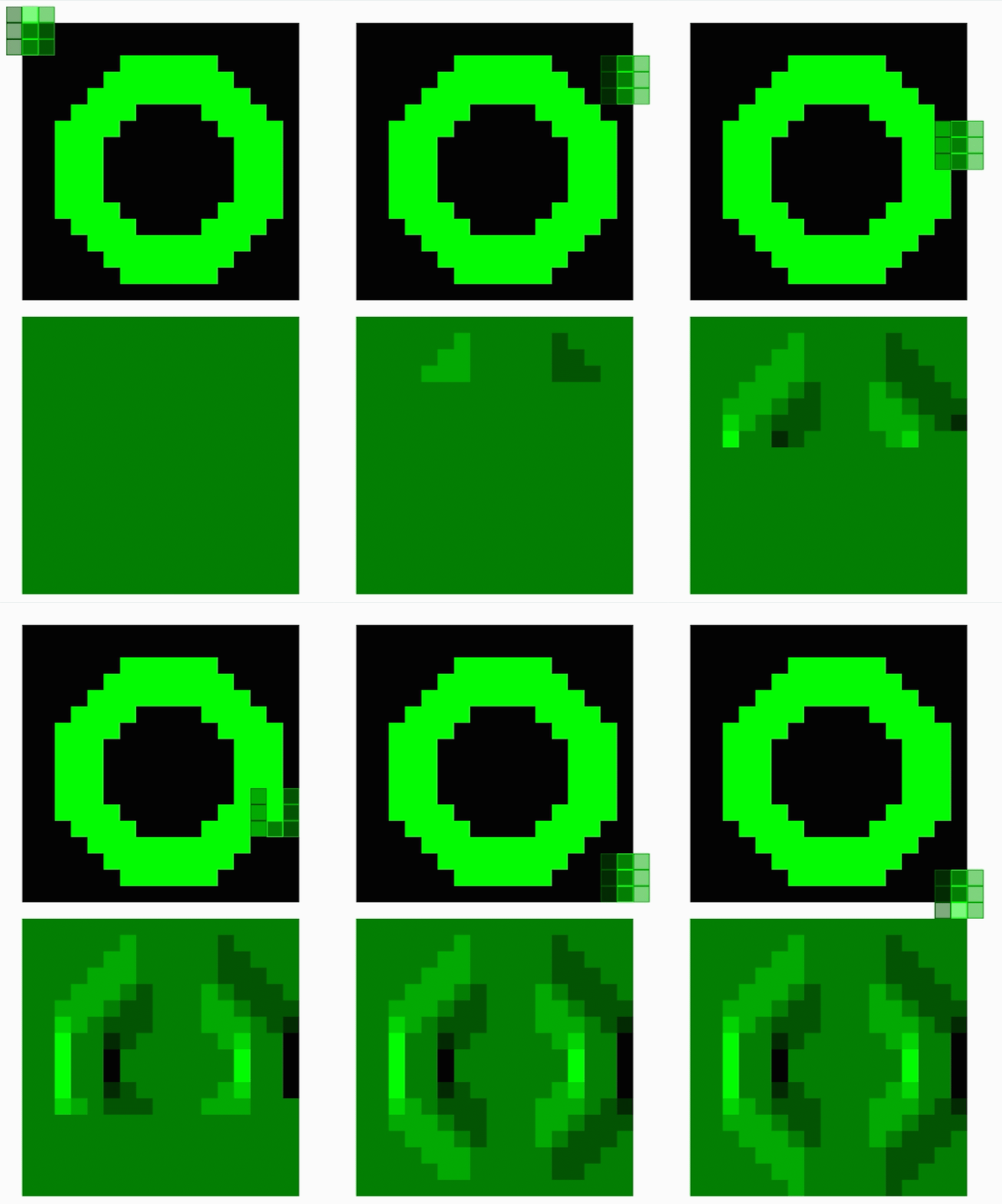
<p>Speaking at a high level, the filter is first compared with the top left corner of the image.
The pixels in the image will most likely have a different color than those in the filter, so we calculate an error value.
This error value is then stored in the top left corner of a new image.
This new image in reality is just a vector of numbers, but we represent it as an image to show where each number comes from.</p>

<!-- Image of filter making first comparison -->

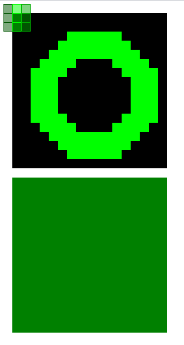
<p><img src="/assets/images/ganintro_convframe.png" alt="Filter" /></p>

<p>Then, we move the filter over by 1 pixel, which is called a <em>stride</em>.
And, rinse and repeat.</p>

<ol>
  <li>Calculate the error</li>
  <li>Store the error in the corresponding square in a new image</li>
  <li>Move the filter to the right. (If at the end of a row, move to the beginning of the next row.)</li>
</ol>

<p>The process of comparing the filter with each section of the image is called <em>convolution</em>.</p>

<!-- Gif of filter making comparisons -->

<p><img src="/assets/images/ganintro_convgif.gif" alt="Filter" /></p>

<p>At the end, we are left with a little image, full of error values.
The parts with the least error tell us where the filter matched the image the most, and the parts with the most error tell us where the filter matched the least.</p>

<p>Just like any other layer, convolutional layers have inputs and outputs.
The input is the initial image, and the output is the image filled with the convolving error data.</p>

<p>Generally, there are only a couple convolutional layers per CNN because they take so much more time to compute.
Plus, once the general patterns are detected, normal neural network layers are able to put two and two together to predict what’s in the image.
For example, if the convolutional layers determined that there was a dog face, a human face, and a long line in the image, the neural network could determine that the image probably depicts a human walking a dog on a leash.</p>

<!-- Someone walking a dog -->

<p><img src="/assets/images/ganintro_dogwalk.jpg" alt="Someone Walking A Dog" /></p>

<h1 id="generative-networks">Generative Networks</h1>

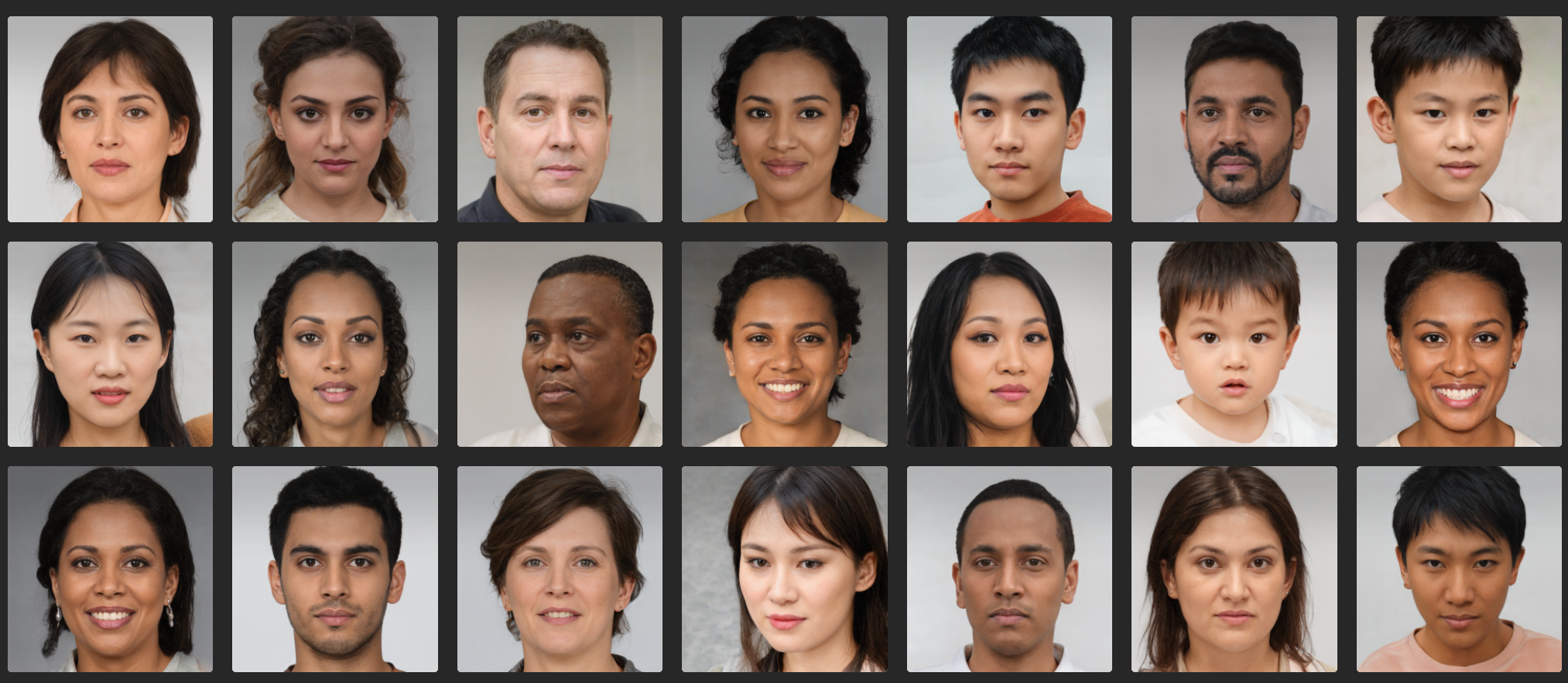
<p>You may have seen images of human faces that don’t exist, but instead were generated by a computer.
Those were created using generative networks.</p>

<!-- Image of computer generated faces -->

<p><img src="/assets/images/ganintro_faces.png" alt="Generated Faces" /></p>

<p>As you know, neural networks have a bunch of input and output values.
We’ve discussed models where the input layer holds an image, but what about the output?
There’s nothing stopping us from making a large output!
(Make sure to also consider other things, like ingredients for a certain recipe, or health statistics for a certain person with a disease)</p>

<p>That’s exactly what a generative network is; a neural network that has a bunch of outputs, possibly to be represented a different way.
(An image, for example.)
Now, it’s common that these generative networks have a bunch of inputs as well.
Let’s think about the theory; if there were only a small amount of inputs, the model wouldn’t be able to generate a large variety of outputs.
Instead, it would be restricted to certain images due to a lack of variety in the inputs.
However, if we had a ton of inputs, we would have to blame the lack of variety on the edge weights inside the network, which would just come down to training.</p>

<p>The set of all input vectors for such generative networks is called the <em>latent space</em>, which has many interesting properties that I won’t be getting into today. Maybe in the future, though.</p>

<h1 id="cnns-as-generative-networks">CNNs as Generative Networks</h1>

<p>There are many, many different types of generative networks, but the one that I’ll be going into are the generative convolutional networks.</p>

<p>The theory is pretty simple, actually.
We just treat the input from the latent space as some type of image, itself.
Then, we can use convolutional layers to not only find and relate certain patterns in the latent space, but also to give different numbers of outputs until we reach the desired image size.</p>

<p>For example, imagine the latent space has 100 dimensions, and we want our output image to be 20x20 pixels large.
We could have a convolutional layer that detects patterns in the latent space, then feeds the output into another layer called a reverse pooling layer.
All you need to know about this layer is that it basically just scales up the image.</p>

<p>Using multiple convolutional layers and upscaling layers, you can eventually land at an output vector size of 400, aka 20x20.</p>

<h1 id="discriminator-networks">Discriminator Networks</h1>

<p>A Discriminator is an essential part of a GAN.
It’s basically a network that takes an image as an input, and has a single output, which is the probability that the image is real or not.
For a basic understanding, that’s all you need to know!</p>

<h1 id="cnns-as-discriminator-networks">CNNs as Discriminator Networks</h1>

<p>It’s a good idea to use convolutional layers in discriminator networks.
Since it’s the discriminator’s job to figure out if the image is real or fake, it needs to be really good at recognizing certain things in the given image.
Luckily, convolutional layers are great at that!
They help networks recognize patterns.</p>

<p>Convolutional layers allow the discriminator networks to predict with more accuracy and less training, due to the pattern-recognition nature of convolution.</p>

<h1 id="duality">Duality</h1>

<p>Finally, we get to understand what a GAN is, as a whole!
GAN stands for Generative Adversarial Network.
We know what a generative network is, so that’s easy to understand.
The adversarial part is the part that makes GANs so revolutional, though.</p>

<p>As you may know, an adversary is like an opponent.
The first thing that may come to your mind about a GAN is a network fighting an adversary.
A strange thought, but one that holds truth nonetheless.
In the case of a GAN, the adversary is actually a second neural network.</p>

<p>A good analogy of a GAN is like an art forger, and an art critic.
It’s the art forger’s job to make art that looks like it’s real, so they can sell it and get rich (or something).
The art critic’s job is to look at a piece of art, and figure out if it is genuine/authentic, or if it has been forged.
The forger and critic have varying levels of accuracy, though.</p>

<p>At the beginning, the forger may make paintings that look like complete garbage.
Obviously, the critic would have an easy time figuring out that it was forged.
But over time, the forger would improve with both feedback from the critic and time spent studying authentic images to imitate them.</p>

<p>Eventually, the forger will become good enough to fool the critic into thinking the fake art was real.
However, after a long hard search, the art critic is able to find a bunch of work by the forger.
After studying said work, the critic is able to distinguish forged artwork from authentic once again!</p>

<p>And the cycle continues.
The forger keeps improving its forging skills while the critic keeps improving its detection skills.
After a while, what we are left with is a very skilled forger and a very skilled critic.
So, if you wanted to buy artwork from a certain artist, but you don’t have the money for it, you could just ask the forger for some!</p>

<p>This is the basic idea behind GANs.
The art forger is the generative network, and the art critic is the adversarial network (aka discriminator).
We train the generative network using the discriminator’s output (probability of being generated) as an accuracy function.
We then train the discriminator by feeding it real images from the dataset (which are classified as real) and fake images from the generator (which are classified as fake).
After many iterations (aka generations/epochs) of training both networks, we should be left with a generative network that is able to somewhat replicate images from our dataset, but they are completely new.</p>

<p>Of course, don’t forget that the dataset doesn’t have to contain images.
It can contain any type of data we want.
Images, 3d models, recipes, medical data, text, audio, etc.</p>

<h1 id="why-gans-are-so-powerful">Why GANs are so Powerful</h1>

<p>The fact that GANs have two different networks both competing against each other and learning from each other at the same time is what makes them so powerful.
If there wasn’t another network to test the accuracy of the other, we would have to rely on only the given dataset for that.
That means, we would need a larger dataset, possibly orders of magnitude larger, to get similar results.
Since there’s a larger dataset to train on, that also means that we would need more computing time.</p>

<h1 id="real-world-examples-of-gans">Real World Examples of GANs</h1>

<p>GANs are so revolutionary that large companies have started testing with them.</p>

<p>NVidia, being a GPU designer, <a href="https://research.nvidia.com/sites/default/files/pubs/2017-10_Progressive-Growing-of/karras2018iclr-paper.pdf">has worked a lot with machine learning algorithms</a> to speed them up.
They are able to generate faces that no one has ever seen before, using GANs.</p>

<p>Google made a machine learning library for easy implementation of GANs.
They call it TensorFlow, and with it comes some of the best resources for actually learning machine learning without learning all of the theory: <a href="https://developers.google.com/machine-learning/gan">the documentation</a>!</p>

<p>There was a <a href="https://www.youtube.com/watch?v=SacogDL_4JU&amp;list=PLrUdxfaFpuuLyYmu__kWChp_F0weDD6yj">series of youtube videos</a> that actually made me aware of machine learning by a guy named Cary Huang.</p>

<p>Another more interactive example is this online <a href="https://generated.photos/face-generator">face generator</a>.
They even reference NVidia’s paper on GANs!</p>

<p>Of course, there are countless other examples in the real world.
You can find those that aren’t listed by just searching interactive GAN (or something).</p>

<h1 id="the-end">The End</h1>

<p>I’m learning about GANs because I plan on using them for a project, which involves generating 3d models using them.
Of course, this means that I’m also a beginner (as of right now) so I may come back to this post and change some things once I know better.
But, I think this post serves as a good introduction to what the theory behind a GAN is.
Anyway, thanks for reading!</p>

<h2 id="good-resources-i-found--have-been-shown">Good Resources I Found / Have Been Shown</h2>

<ul>
  <li><a href="http://3dgan.csail.mit.edu/">MIT Paper on 3D GANs</a></li>
  <li><a href="https://machinelearningmastery.com/how-to-develop-a-generative-adversarial-network-for-an-mnist-handwritten-digits-from-scratch-in-keras/">Jason Brownlee’s Basic GAN with MNIST</a></li>
  <li><a href="https://machinelearningmastery.com/what-are-generative-adversarial-networks-gans/">Jason Brownlee’s Basic Theory Behind GAN</a></li>
  <li><a href="https://www.youtube.com/watch?v=YRhxdVk_sIs">DeepLizard’s CNN Overview</a></li>
  <li><a href="https://www.tensorflow.org/tutorials/generative/dcgan">TensorFlow’s GAN tutorial</a></li>
  <li><a href="https://deeplizard.com/learn/video/m0pIlLfpXWE&gt;">DeepLizard’s Great Deep Learning Youtube Series</a></li>
  <li><a href="https://www.deeplearningbook.org/">The Deep Learning Book</a></li>
  <li><a href="https://github.com/NVlabs/stylegan">NVLabs StyleGAN Documentation</a></li>
  <li><a href="https://www.fast.ai/">FastAI</a></li>
</ul>]]></content><author><name></name></author><category term="post" /><category term="machine-learning" /><summary type="html"><![CDATA[What is a neural network? You may have heard of neural networks before, and you may know that they mimic brains. Many people’s knowledge on neural networks falters after that. However, I’m here to provide a basic overview of what they are, and how they work.]]></summary></entry><entry><title type="html">An Overview of FAT12</title><link href="https://oriont.net/posts/fat12-overview" rel="alternate" type="text/html" title="An Overview of FAT12" /><published>2021-04-14T00:00:00+00:00</published><updated>2021-04-14T00:00:00+00:00</updated><id>https://oriont.net/posts/fat12-overview</id><content type="html" xml:base="https://oriont.net/posts/fat12-overview"><![CDATA[<p>What is FAT12?
FAT12 stands for File Allocation Tables, 12.
It was introduced in 1977 (almost 50 years ago!) and has many descendents, such as FAT16, FAT32, and exFAT.
It’s a file system that was used in early computers, and is can likely be found on any floppy disk you come across.
As the first file system that I’ve ever delved into, I can say that it’s fairly simple to learn.</p>

<p>Many people have tried to explain this, but in my experience, they all miss some small portion.
With that in mind, let’s start learning!</p>

<h1 id="quick-overview-of-storage-devices">Quick Overview of Storage Devices</h1>

<p>I’d like to start off with what storage devices actually do, because I always accidentally confuse people by assuming they know this.
A storage device is literally something that holds data. This can be a book, a document, a drawing, a harddrive, etc.
Anything that can hold information (which is literally everything) can be a storage device.
However, it’s much easier for computers to interface with storage devices that hold data in terms of 1’s and 0’s.
Examples of these are: Floppy disks, Hard disks/drives, SSDs (Solid State Drives), Thumb drives (USB-flash storage), M.2 SSDs.
There are countless types.
However, all you really need to know about them is that they hold a sequence of 1s and 0s in a specific order, which we can change whenever we want.</p>

<p>Computers are made in a way such that it’s much easier to deal with 8, 16, 32, or 64 bits at a time.
These are the most common, but most powers of 2 (greater than 64) are also common.
A sequence of 8 bits is called a <em>byte</em>.
The capacity of most computer-interfaceable storage devices are measured in bytes.
For example, the computer you have might have 250 gigabytes of storage.
As you might know already, <em>giga</em> means 1 billion, so you have <em>250 billion</em> bytes of memory at your disposal!
The prefix <em>giga</em> comes from the orders of magnitude prefixes for SI units, which you can find at <a href="https://www.thermofisher.com/us/en/home/references/ambion-tech-support/rna-tools-and-calculators/orders-of-magnitude-prefixes-for-si-units.html">this link</a>.</p>

<p>There is also another type of prefix, which is very similar to the SI prefixes, but it’s in powers of 2.
You can find a table for them <a href="https://en.wikipedia.org/wiki/Byte#Multiple-byte_units">here</a>, and notice how similar they are to the SI prefixes!
This is often a source of confusion. I only learned about them recently as well!
So, if you ever see an ‘i’ in the middle of a byte unit, just know it’s in binary.
Meaning, 1 KB = 1000 B, but 1 KiB = 1024 B. (Kilobyte vs Kibbibyte)
Generally, they are very similar, so it usually doesn’t matter, but we’ll be getting into very specific amounts of bytes very soon, so it’s good to know the difference.</p>

<h1 id="partitioning">Partitioning</h1>

<p>It’s kind of ambiguous when defining a partition of a disk, without using ‘operating system’, so I’ll define it in the mathematical sense.
Imagine you have a set of numbers \(\{1, 2, 3, 4, 5, 6, 7, 8, 9, 10\}\).
A partition of this set is a <em>set of sets</em> where the numbers contained in those inner sets aren’t duplicated at all, and they make up the whole original set.
For example, these <em>are</em> partitions of our original set:</p>

\[\{ \{1, 2\}, \{3, 4\}, \{5, 6\}, \{7, 8, 9, 10\} \} \\
\{ \{1, 10\}, \{9, 8\}, \{2, 7\}, \{3, 4\}, \{5, 6\} \} \\
\{ \{1, 2, 3, 4, 5, 6, 7, 8, 9, 10\} \}\]

<p>And these <em>are not</em> partitions of our original set:</p>

\[\{ \{1, 2\}, \{3, 4\}, \{5, 6\} \} \\
\{ \{1, 10\}, \{9, 7, 8\}, \{2, 7\}, \{3, 4\}, \{5, 2, 6\} \}\]

<p>The first one is missing numbers \(7-10\) and the second one has an extra 7 and 2.
Disk partitioning is very similar.
We have a disk with x bytes on it, and we can <em>partition</em> it so that the first half and second half are different <em>partitions</em>.
Notice how “partition” can be used as both a verb and a noun.
Also notice how each partition (n) has <em>no overlapping</em> with other partitions, and the <em>sum of all partitions makes up for the whole disk space</em>.</p>

<p>For the purposes of simplicity, I won’t be using any file system partitioning, which is where partitions of the disk are used for <em>completely different filesystems.</em>
We’ll treat the disk like it’s one big partition, and our filesystem will take up the whole partition.
However, that’s not to say we won’t be using any partitioning!
It’s actually very important.
For example, for this specific filesystem (FAT12), we need a section which tells us which parts of the disk are free to store data in (which, by the way, is in a different section!)
Also, since disk partitioning is usually associated with having a different filesystem on each partition, I’ll call them sections from now on.</p>

<h1 id="structure-of-fat12">Structure of FAT12</h1>

<p>There are a couple different sections in FAT12. Here’s a list of them, in the order that they appear on the disk:</p>

<ul>
  <li>“Reserved” Section</li>
  <li>File Allocation Tables (hey, that’s the name of the filesystem!)</li>
  <li>Root Directory</li>
  <li>Data Section</li>
</ul>

<p><img src="/assets/images/fat12_sections.png" alt="Fat12 Sections" /></p>

<p>Each of these sections also is split up, but these are the basic ones that we need to remember.
In FAT12, the sections are split up slightly different to how it’s split up in FAT16 and FAT32, so from now on, I will only be talking about FAT12.
However, they are similar enough that later, we can use the base understanding that we are building right now to continue.</p>

<p>One term I need to define before we continue, is a sector.
In the file system sense, a sector is 512 bytes.
Apparently this is configurable, however we’re going to keep it at 512 bytes for simplicity.
From now on, always assume a sector is 512 bytes.
The other term I need to define is a cluster.
A cluster is just a group of adjacent sectors of a specific length.
Again, for simplicity, I’ll be using 1 sector per cluster, meaning our math should simplify a bit.
The only place where we’d rather use clusters than sectors is in the data section, as mentioned in the list above.
Let’s get into what each section actually does.</p>

<h1 id="reserved-section">Reserved Section</h1>

<p>The first section is only 1 sector long. Notice how it’s a sector, and not a cluster.
That’s because we’re in the reserved section, not the data section.
The first sector of a disk is a special sector called the “boot sector”.
It contains machine code that your computer automatically loads when you turn it on, and it runs that code which is supposed to load your operating system.
It’s very interesting, but it’s also a topic for another post.</p>

<p>One notable thing about the boot sector is a group of bytes called the “Bios Parameter Block”, or BPB for short.
The parameter block is full of specifically ordered bytes in an exact length to configure things such as how big a sector is, or how many sectors long a cluster is, or how many entries can be in the root directory, etc.
However, we won’t need to worry about that in this post, since 1. This is all conceptual (for now), and 2. We will define this stuff as we go.</p>

<p>Wow, first section out of the way! That was easy, right?
As it turns out, that was the easeist one by far. Onwards!</p>

<h1 id="the-data-section">The Data Section</h1>

<p>I’ll explain the data section before the file allocation tables, since it’s the second easiest section to understand.
The data section is, as the name suggests, the section where we store all of our data.
So, if we have a text file, the actual ascii/utf-8 bytes representing the text would be stored here.
If you had an image, it would also be stored here, in binary format. (That may entail each pixel being stored as a certain sequence of bits)
Any file that you would have on your computer is stored in this section of the disk.</p>

<p>Since we have to store all of our files here, this is the biggest section, by far.
<a href="https://en.wikipedia.org/wiki/Linked_list#:~:text=In%20computer%20science%2C%20a%20linked,which%20together%20represent%20a%20sequence.">According to wiki,</a> the maximum volume size for a disk using the FAT12 system is 32 MiB.
I haven’t defined what a volume is, so just understand that the maximum size of the data section can be 32 MiB minus the reserved section, minus the file allocation tables.
That turns out to still be really close to 32 MiB.</p>

<p>You may ask, “Why would anyone want to use a file system that can only support 32 MiB? I have a single image file that’s larger than that!”
I would tell you that that’s a good question!
But, remember, this file system was introduced in 1977!
Back then, <a href="https://www.wired.com/1997/01/did-gates-really-say-640k-is-enough-for-anyone/#:~:text=Gates%20said%20once%20that%20'640K,ever%20need%20on%20a%20computer.&amp;text=Gates%20said%20that%20640K%20of,a%20computer%20would%20ever%20need.">some people thought that no one would ever need more than 640k of memory</a>, but today, even the lowest end computers have at the very least 2 GB of memory.
(Memory is not the same thing as storage, but my analogy still stands.)
Later, we can upgrade to FAT16 or FAT32, which can hold more data.</p>

<p>One other thing to note is that directories are actually stored as files.
We can explore how this works later, but just know that it’s stored as a file, containing “links” to all of the files that it contains.</p>

<p>The last thing you should know about the data section is that the very first file is</p>

<h1 id="file-allocation-tables">File Allocation Tables</h1>

<p>The file allocation tables are what characterize this file system, and is also the hardest section to understand.
This is essentially a <a href="https://en.wikipedia.org/wiki/Linked_list#:~:text=In%20computer%20science%2C%20a%20linked,which%20together%20represent%20a%20sequence.">linked list</a> which tells us where our files are and which parts of the disk are free for us to put more data in.</p>

<p>If you don’t understand how linked lists work, I urge you to do some research.
They are a common data structure used for making dynamically sized lists, and can be modified slightly to make trees, graphs, and even weighted trees and graphs.</p>

<p>Anyway, the FAT linked list is all in binary.
You may be wondering how this works, and rightfully so! (It’s actually really interesting!)
Essentially, each entry in the list is exactly 12 bits. (Hence the name of FAT<em>12</em>)
We’ll think of the table as 12 bit entries for now, but when we get into how we would implement this in the real storage device, we will need to start thinking about 12 bits as 1.5 bytes.
(It’s pretty icky…)</p>

<h2 id="example-1">Example 1</h2>

<p>Here’s an example of how a file is stored.
At first, every entry is set to 0.
This is a reserved value, which means “hey computer, there’s no useful data here, so you can store whatever you want here!”
It indicates free space.
In order to find <em>where</em> on disk we should store our file, we need to find the first FAT entry that is free (AKA equal to 0)</p>

<!-- Image of first free FAT entry -->

<p><img src="/assets/images/fat12_entries.png" alt="First Free FAT Entry" /></p>

<p>The <em>index</em> of this FAT entry is equal to the <em>index</em> of a cluster in the <em>Data Section</em>.
This is the first cluster that we will use to store our data in.</p>

<!-- Image explaining this -->

<p><img src="/assets/images/fat12_entries_clusters.png" alt="FAT Entries Clusters" /></p>

<p>Now, let’s imagine that our file is 100 bytes long.
Since a cluster is equal to 1 sector, and a sector is equal to 512 bytes, we have plenty of space to store our file in here!
So, let’s just copy the 100 bytes of our file into the cluster.</p>

<p>Now, our entire file is stored in the data section.
However, our computer will never know that a file is stored there, since we never updated the FAT!
Remember, it’s still set to 0, which means “this space is free!”</p>

<p>The way we assign the FAT entry is by giving it the index of the <em>next</em> cluster of the file.
BUT, since our file <em>only takes up 1 cluster</em>, we don’t have anything to put here!</p>

<p>This is where another reserved value comes into play.
A value of 0xFFF in hex will signify that this cluster is the <em>last cluster of the file</em>.
Effectively, this signifies the <em>EOF</em>. (End Of File)</p>

<p>So, we’re done! That was pretty easy!
Before I answer any other questions on how the computer may <em>find</em> that file, let’s try another one.</p>

<h2 id="example-2">Example 2</h2>

<p>Imagine our file is 1536 bytes long exactly.
Well this is a nice number, because it’s exactly \(512 * 3\) bytes!
This means that it’s exactly 3 clusters long!
(Remember, 1 sector = 1 cluster = 512 bytes)</p>

<p>We always start with the first cluster.
So, first we find the next free entry in the FAT. (Equal to 0)</p>

<p>Then, we get the <em>index</em> of that entry, and match it up with the cluster who has the same <em>index</em>.
We store the first cluster of our data into this cluster that we just specified.
Next, we would store something in the FAT entry.
Remember, we store the <em>index of the *next* entry</em> in the FAT.
But, seeing as we don’t have a <em>next</em> entry yet, let’s keep this current one in mind and move on.</p>

<p>Now, we need to store the next cluster of our data.
Let’s find a new free FAT entry.</p>

<!-- Image of free entry -->

<p><img src="/assets/images/fat12_entries.png" alt="First Free FAT Entry" /></p>

<p>Now, let’s find the cluster with the same <em>index</em> of that entry!</p>

<!-- Image of free cluster -->

<p><img src="/assets/images/fat12_entry_cluster.png" alt="Entry Cluster" /></p>

<p>Now, we can store the <em>next</em> cluster of our file in here.
That would be bytes 513-1024, since bytes 0-512 are stored in the first cluster we had.
And next, we need to fill up the FAT.
Think back to last time: we now have that “next entry” ready!
That “next entry” will just be the <em>index</em> of the current cluster we’re on.</p>

<p>So, let’s go back to the <em>old index</em>.
Last time, we wanted to store the <em>next index</em>, but we didn’t get it yet, but now we have it!
So, let’s store the <em>current index</em> <em>in</em> the <em>old index</em>.</p>

<!-- Image of the FAT now -->

<p><img src="/assets/images/fat12_entry_cluster_2.png" alt="Entry Cluster" /></p>

<p>Phew, that was a lot of emphasized text! But, we aren’t done!
That was only 2 clusters of the 3 that our file requires.
Remember, it was 3 clusters long.</p>

<p>So, let’s find the next free FAT entry.
Then, let’s find the cluster with the same index as that FAT entry.
Now, let’s store bytes 1025-1536 (the 3rd cluster) in there. That’s the last of our data!
Last, don’t forget to update the FAT table!
So, let’s store the <em>current index</em> <em>in</em> the <em>old index</em>.</p>

<!-- Image of the FAT now -->

<p><img src="/assets/images/fat12_entry_cluster_3.png" alt="Entry Cluster" /></p>

<p>And finally, since this is the last cluster of the file, let’s store the special reserved <em>EOF</em> value in the <em>current index</em>.</p>

<!-- Image of the FAT now -->

<p><img src="/assets/images/fat12_entry_cluster_4.png" alt="Entry Cluster" /></p>

<h2 id="to-generalize">To Generalize</h2>

<p>That’s probably the most confusing part of FAT.
If you got lost, I encourage you to read that second example again, and definitely look at the pictures for guidance.
We can be generalize this method in a small algorithm.</p>

<p>For each cluster in the file we want to store:</p>

<ol>
  <li>Get the first free/empty FAT entry</li>
  <li>Store the current file cluster in the cluster <em>at the index of current FAT entry</em></li>
  <li>Set <em>current</em> FAT entry to EOF (0xFFF)</li>
  <li>Set <em>previous</em> FAT entry to <em>index of current</em> FAT entry (if there <em>is</em> a previous FAT entry)</li>
</ol>

<p>Notice how I made step 3 set the current entry to EOF.
This is actually a small shortcut that I just thought of, which makes it so that we don’t have to check if the current cluster is the last cluster in the file, and also allows us to simplify our <code class="language-plaintext highlighter-rouge">find first free entry</code> algorithm.
If you think about it, when we are finding the next free entry, in the examples above, the last entry is also set to 0, so we have to purposefully skip that one.
If we set it to an EOF, we won’t have to take that into mind.</p>

<h1 id="reading-a-file">Reading a File</h1>

<p>Now, let’s try reading a file given the index of the first cluster.</p>

<p>Well, we know that the index of the cluster is attached to the index of the FAT entry, so let’s get that FAT entry.
We also know that each FAT entry will point to the index of the next FAT entry for the file, which also is the index of the next cluster.
When we come across a FAT entry that is equal to 0xFFF, we know that’s the end of the file, so we can copy the current cluster and end the search.</p>

<h2 id="to-generalize-1">To Generalize:</h2>

<p>Until we reach an <em>EOF</em> entry:</p>

<ol>
  <li>Copy the cluster at the index of the current FAT entry into memory</li>
  <li>Set the current FAT entry to the one <em>stored</em> in the current FAT entry</li>
</ol>

<p>Simple!
I don’t know much about other filesystems, but even if I did, this would probably seem very easy.</p>

<h1 id="directories">Directories</h1>

<p>Think about this from a larger standpoint.
When we turn on our computer, how does it know which code to run?
Well, we’d determine that if we were writing the <em>bootloader</em>.
(Remember I mentioned that earlier for the reserved section?)
We’d want a system of easily grouping files for easy access and organization.
This is exactly what directories are for!</p>

<p>Let’s talk about directories for a second.
As you may know already, a directory is like a manilla folder, if files were paper documents.
It’s just a way to group files.
In the FAT systems, directories are actually stored <em>as</em> files!
This makes it a lot less complicated and more generalized.
So, to read the file and find all of the clusters in the file, we’d read the FAT table <em>exactly the same way for any other file</em>.</p>

<p>Imagine we performed the file read method on a directory.
Now that we have the directory in memory, how do we find the files inside?
Well, the directory file is just full of 32 byte <em>directory entries</em>.
If you have experience with pointers in C, each directory entry is like a pointer to the file, along with attributes.
Every byte of the 32 bytes is used for something, including the filename, file extension, attributes, timestamps, the first cluster of the file, file size, and if this entry is actually a <em>subdirectory file</em>.
If you want to see exactly which bytes are used for what, <a href="https://www.eit.lth.se/fileadmin/eit/courses/eitn50/Literature/fat12_description.pdf">I recommend you look at page 5 of this document</a>.
In fact, read the whole thing!
It was one of the documents <em>I</em> used to learn FAT12.</p>

<p>One thing I noticed, which was kind of funny, was that the file size is 32 bits long.
That means, it’s possible to have 4 GB files in FAT12, even though the entire file system can’t be larger than 32 MB!
In FAT32, the max file size <em>is</em> 4 GB, so eventually we can take advantage of all of those bits.</p>

<h2 id="anyway">Anyway</h2>

<p>To get all the files in a directory, we split it into 32 bit <em>directory entries</em>.
The file name is the first 11 bytes, and the first cluster of the file is in bytes 26-27.
Notice the first cluster is 2 bytes long, even though FAT entries are only 1.5 bytes long.
In FAT12, the last 4 bits of those 2 bytes are just never used.
So, to get a file by name, we can compare the first 11 bytes of each entry to the name we are looking for.
If the names match, we can load the file using the first cluster in bytes 26-27.
Also very simple!</p>

<h2 id="the-root-directory">The Root Directory</h2>

<p>Generally, the root directory is 14 sectors long.
Again, this is configurable in the BPB (Bios Parameter Block), but for the purposes of convention, we’ll keep it at 14.
Since each directory entry is 32 bytes long, and each sector is 512 bytes long, there can be 16 entries per sector.
The root directory has 14 sectors * 16 entries per sector, which is 224 entries.</p>

<p>Notice how I was talking in terms of sectors and not clusters.
This is because in FAT12, the root directory is kind of awkward.
<em>It’s not actually in the data section</em>.
It’s located right after the FAT section, and right <em>before</em> the data section.</p>

<!-- Picture of that -->

<p><img src="/assets/images/fat12_sections.png" alt="FAT12 Sections" /></p>

<p>So, as you can see, reading the root directory will be <em>slightly</em> different than reading any other directory.
In reality, getting stuff from the root directory is actually slightly easier.
For one, it’s always 14 sectors long, and it’s always in a specific location (right after the FAT section), so there’s no need to read the FAT table.
But, since it’s not in the data section, we’ll need to calculate the sector number slightly differently.
(We’d just <em>not</em> add the 14 sectors in the root directory, like we would for the data section, since it’s located <em>after</em> the root directory.)</p>

<p>Having a root directory in a constant place allows us to structure <em>all of our files</em> in a consistantly locatable tree.
What I mean by this, is that we can make subdirectories in the root directory and store files in there, which emulates a tree structure.
This allows us to traverse the tree to find a file at a specific path!
That’s useful for loading system code files into memory to run, which will allow us to build even more tools to explore the files.</p>

<h1 id="the-end">The End</h1>

<p>That’s essentially all you need to know to get started on building your own FAT12 implementation.
Obviously, that’s not all there is to know about FAT12.
There are plenty of limitations that I haven’t discussed.
I also didn’t discuss many of the file attributes, many of which can be considered as important.
I’ll likely make more in-depth posts about more specific parts of the FAT12 system in the future.</p>

<p>If you’re interested, I’m making a FAT12 implementation in rust right now.
I’m using it as a project to both improve at rust and FAT12.
It’s a shell that you can copy files from the host OS to a FAT12 disk image, which I can then use to run on a VM emulator.
If you are interested in it’s progress, you can <a href="https://github.com/eoriont/fat12-image-driver">check out its GitHub page here</a>, and you can <a href="https://www.twitch.tv/eoriont">watch my occasional streams on twitch</a></p>

<p>If you spotted an error in this post, or have something that you’d like to add, please make a github issue or pull request, as linked to in the footer.</p>

<p>Thanks for reading!</p>]]></content><author><name></name></author><category term="post" /><category term="fat12" /><summary type="html"><![CDATA[What is FAT12? FAT12 stands for File Allocation Tables, 12. It was introduced in 1977 (almost 50 years ago!) and has many descendents, such as FAT16, FAT32, and exFAT. It’s a file system that was used in early computers, and is can likely be found on any floppy disk you come across. As the first file system that I’ve ever delved into, I can say that it’s fairly simple to learn.]]></summary></entry><entry><title type="html">Creating a live newton fractal using JS + WebGL</title><link href="https://oriont.net/posts/newton-fractal" rel="alternate" type="text/html" title="Creating a live newton fractal using JS + WebGL" /><published>2021-02-13T00:00:00+00:00</published><updated>2021-02-13T00:00:00+00:00</updated><id>https://oriont.net/posts/newton-fractal</id><content type="html" xml:base="https://oriont.net/posts/newton-fractal"><![CDATA[<p>Long story short: if you want to see the end product, then click on the following link:</p>

<p><a href="https://oriont.net/newtonfractal">https://oriont.net/newtonfractal</a></p>

<h1 id="in-the-beginning">In the Beginning</h1>

<p>A long time ago, I made a newton fractal simulator using javascript with <code class="language-plaintext highlighter-rouge">p5.js</code>.
It worked, but it was sloooooow. You can find it at <a href="https://oriont.net/newtonfractal_old/">this link</a> to see for yourself.</p>

<p>I used all the same methods I used in this new version, except the technologies I use are different, which sped up the program a LOT.</p>

<h1 id="whats-newtons-method">What’s Newton’s Method?</h1>

<p>Newton’s method is a way of <em>approximating</em> the roots of a function.
For example, given the function \(f(x) = x^2 - 1\), the seasoned mathmatician would be able to tell you that the roots are \(1\) and \(-1\).
They’d be correct, but how did they get there?</p>

<p>Well, simple. You could just factor it out into \((x-1)(x+1)\) and use the roots of each factor, or you could use the quadratic formula,
etc. However, what if you can’t find the roots so easily, like \(f(x) = x^7 + 5x^4 + 3x - 1\)? In this case, you would use the Newton-Raphson method, also known as just “Newton’s method.”</p>

<p><img src="/assets/images/newtonfractal_graph1.png" alt="Image of Graph" /></p>

<p>First, let’s take a look at the graph of \(f(x)\). Let’s take a random point on the graph, say, \((0.837, 4.253)\). Taking the derivative at that point will yield:</p>

\[\dfrac{\text{d} f}{\text{d} x} = 7x^7 + 20x^3 + 3 \\
f'(0.837) \approx 17.134\]

<p>Now, how can we get to the closest zero from here? Using deductive reasoning, one can infer that if the slope is positive, then the root must reside at a lower value of x, and if the slope is negative, it must be at a higher x.</p>

<p>What do I mean by this? Well, take a look at the following graph, which has 3 real zeros:</p>

<p><img src="/assets/images/newtonfractal_graph.png" alt="Image of Graph" /></p>

<p>Now, take any arbitrary point (the further away from for the local minima/maxima, the better. I’ll get to that in a bit.) Now, visualize the tangent line of that point. That tangent line will have a positive slope (pointing up-right) or a negative slope (pointing down-left). Now, take a look at the closest zero. You might notice, that <em>usually</em>, the zero of the tangent line is closer to the actual zero, than \((x, 0)\), (x being the x coordinate of your arbitrary point). Why is this?</p>

<p>Well, it’s because the tangent line can be thought as an <em>approximation</em> of the complicated line. When we are talking about approximations, <em>pretty much anything</em> can be an approximation of <em>pretty much anything else</em>. (That’s not to say that they are <em>good</em> approximations). We can treat it as an approximation because it has a zero, which is what we’re looking for.</p>

<p>Now, this approximation (tangent) line that we have, will give us our approximated zero! Since the equation of the tangent line can be modeled (in point-slope form) as:</p>

<p>\(y - f(x_1) = m (x - x_1)\),</p>

<p>Where \((x_1, f(x_1))\) is the point of intersection, and \(m\) is the slope (aka derivative) of the line, we can model the <em>actual</em> tangent line as:</p>

\[y - f(x_1) = f'(x_1) (x - x_1)\]

<p>Now, let’s solve for the y intercept. The y intercept is a point on the line where \(y=0\), so we can set \(y=0\) and solve for x. We don’t set \(f(x_1)\) to zero, because that’s the thing we’re trying to get closer to zero! (If we could just set \(f(x_1)\) to zero, it’d be the same as finding the <em>actual</em> zeros, meaning we go back to the quartic functions or mega factoring or some other method.)</p>

<p>We have:</p>

\[y = 0 \\
0 - f(x_1) = f'(x_1) (x - x_1) \\
-\dfrac{f(x_1)}{f'(x_1)} = x - x_1 \\
x = x_1 - \dfrac{f(x_1)}{f'(x_1)} \\\]

<p>Now, we have an approximation for the y-intercept! It’s modeled as:</p>

\[(x_1 - \dfrac{f(x_1)}{f'(x_1)}, 0)\]

<p>Coming from \((x, y)\), where \(x\) is what we just derived, and \(y=0\), which was the assumption that we made in order to derive it.</p>

<p>Now what? We have an approximation of the y-intercept, but what if it’s bad? What if we want to make it slightly better? Let’s use this method again, but in order for the next approximation to be better, we need to make sure that the initial point we choose is closer than the last one. From the first approximation, we got a point closer to the y-intercept than our initial point, so let’s use that as a starting point.</p>

<p>First, let’s make an equation for the y-intercept approximation, since we’re going to be reusing it.</p>

\[x\_{n+1} = x_n - \dfrac{f(x_n)}{f'(x_n)}\]

<p>I use the expression we got as the y-intercept approximation, except instead of \(x_1\), I use \(x_n\), since we are performing this operation more than once. And I set it equal to \(x_{n+1}\) since it’ll be used to make the <em>next</em> approximation.</p>

<p>To get the starting point, let’s use the x value as the approximation, which then allows us to get the y value using \(f(x)\). So, our next starting point is: \((x_2, f(x_1))\). Running the whole approximation process again, we get:</p>

\[(x_3, f(x_2))\]

<p>Where \(x_3\) is the new approximated y-intercept, calculated using \(x_{n+1}\), or in this case, \(x_{2+1}\). You might be able to see where this is going. Doing this process infinitely many times will <em>theoretically</em> give you the correct y-intercept for a function! But, it can only give <em>one</em> y-intercept at a time.</p>

<p>Notice, if you start at a different point on the graph, the process might converge on a <em>different</em> y-intercept. This is because the tangent line is closer to another y-intercept than the first one.</p>

<p>To give it a formal definition, let \(f(x)\) be a differentiable function, and \((x_0, f(x_0))\) is an arbitrary starting point. Use the following function:</p>

\[x\_{n+1} = x_n - \dfrac{f(x_n)}{f'(x_n)}\]

<p>to approximate a root. Higher values of \(n\) will yield better approximations of the root.</p>

<h1 id="when-newtons-method-fails">When Newton’s Method Fails</h1>

<p>Earlier, I mentioned that you shouldn’t choose a point close to the local minima/maxima. Let’s try it out to see what I mean. Take a point right next to the critical point, and let’s make an approximation. I’ll just do it visually:</p>

<p><img src="/assets/images/newtonfractal_graph2.png" alt="Graph with Tangent" /></p>

<p>You’ll notice, the tangent line is almost horizontal, meaning the y-intercept’s magnitude is going to be very large. Obviously, this y-intercept is going to yield a much worse approximation than the beginning. However, with this function, if we continue using newton’s method, we are actually able to redeem ourselves with an okay approximation soon enough.</p>

<p>If we were to start <em>on</em> the critical point, however, newton’s method would diverge. This is because the slope is 0, meaning the next point would be:</p>

\[x_1 = x_n - \dfrac{f(x_n)}{f'(x_n)} \\
= x_n - \dfrac{f(x_n)}{0} \\
= - \infty\]

<p>This is one example of newton’s method diverging.</p>

<p>Some functions aren’t friendly with newton’s method. Take, for example,</p>

\[f(x) = \begin{cases}
\sqrt{x}, \quad \text{for} x \geq 0 \\
-\sqrt{-x}, \quad \text{for} x &lt; 0 \\
\end{cases}\]

<p><img src="/assets/images/newtonfractal_graph3.png" alt="Graph of Cases" /></p>

<p>Using newton’s method on this function, starting at any point except for the y intercept, will always diverge. You would have to use a different method to approximate the roots.</p>

<h1 id="applications-of-newtons-method">Applications of Newton’s Method</h1>

<ul>
  <li>Approximating Non-linear functions</li>
</ul>

<p>As the example above showed, what if you want to calculate the roots of a really <em>gnarly</em> function, such as \(y = x^10 + x^9 + x^8 + x^7 + 3x^6 + 3x^5 + x^4 - x^3 + 3x^2 - 8x + 1\)? You could either spend a bunch of time finding factors, or just use newton’s method.</p>

<ul>
  <li>Optimization</li>
</ul>

<p>In calculus, optimization problems are when you want to find critical points of a function. The derivatives/slopes at critical points are going to be 0, so you could use newton’s method on the derivative, in order to find said points.</p>

<ul>
  <li>Cool fractals</li>
</ul>

<p>This is what we’ll be exploring more today. It turns out that newton’s method works with complex numbers as well, so functions \(f(z)\) can be used to approximate zeros. Interestingly, newton’s method tends to jump around when working with complex numbers, due to the fact that certain operations with with imaginary numbers (i.e. squaring) will produce real numbers, and real numbers can become complex (through \(\sqrt{-x}\)). This means certain groups of points will converge to certain roots using newton’s method, and other groups will converge to other roots. This is what makes for a cool fractal effect.</p>

<h1 id="writing-newtons-method-in-code">Writing Newton’s Method in Code</h1>

<p>Let’s really quickly go over how we could go about writing newton’s method in code. We know how the math works, so now all we have to do is create a function.</p>

<p>The inputs should include: \(f\), \(f'\), \(x_0\), and the amount of steps we should take. This ‘steps’ input is actually just the value of \(n\) we would like our code to stop at, since it could keep going forever. Usually, 25-50 gives <em>pretty</em> good approximations. Right now, it looks like this:</p>

<div class="language-js highlighter-rouge"><div class="highlight"><pre class="highlight"><code><span class="kd">function</span> <span class="nx">newtonsMethod</span><span class="p">(</span><span class="nx">f</span><span class="p">,</span> <span class="nx">fp</span><span class="p">,</span> <span class="nx">x0</span><span class="p">,</span> <span class="nx">steps</span><span class="p">)</span> <span class="p">{</span>
  <span class="c1">// Code goes here!</span>
<span class="p">}</span>
</code></pre></div></div>

<p>Now, we have to repeatedly apply newton’s method to the variable \(x_n\), <code class="language-plaintext highlighter-rouge">steps</code> amount of times. We can use a simple <code class="language-plaintext highlighter-rouge">for</code> loop for that. Then, we just return \(x_n\). Our function now looks like this:</p>

<div class="language-js highlighter-rouge"><div class="highlight"><pre class="highlight"><code><span class="kd">function</span> <span class="nx">newtonsMethod</span><span class="p">(</span><span class="nx">f</span><span class="p">,</span> <span class="nx">fp</span><span class="p">,</span> <span class="nx">x0</span><span class="p">,</span> <span class="nx">steps</span><span class="p">)</span> <span class="p">{</span>
  <span class="kd">let</span> <span class="nx">xn</span> <span class="o">=</span> <span class="nx">x0</span><span class="p">;</span>
  <span class="k">for</span> <span class="p">(</span><span class="kd">let</span> <span class="nx">n</span> <span class="o">=</span> <span class="mi">0</span><span class="p">;</span> <span class="nx">n</span> <span class="o">&lt;</span> <span class="nx">steps</span><span class="p">;</span> <span class="nx">n</span><span class="o">++</span><span class="p">)</span> <span class="p">{</span>
    <span class="nx">xn</span> <span class="o">-=</span> <span class="nx">f</span><span class="p">(</span><span class="nx">xn</span><span class="p">)</span><span class="o">/</span><span class="nx">fp</span><span class="p">(</span><span class="nx">xn</span><span class="p">);</span>

    <span class="c1">// This is short for:</span>
    <span class="c1">// let xn1 = xn - (f(xn)/fp(xn));</span>
    <span class="c1">// xn = xn1;</span>
  <span class="p">}</span>
  <span class="k">return</span> <span class="nx">xn</span><span class="p">;</span>
<span class="p">}</span>
</code></pre></div></div>

<p>We now have a simple function for approximating the zeros of a function, given that function, its derivative, a starting point, and an approximation depth (<code class="language-plaintext highlighter-rouge">steps</code>). Now, let’s try it out!</p>

<p>As stated at the beginning of the post, the zeros for the function \(f(x) = x^2 - 1\) are: \(x = \pm 1\). Let’s see if our newton’s method function can calculate the zeros. We’ll set the starting point as, say \(x_0=15\). <em>Note:</em> we won’t set \(x_0\) to 0, because that’s a critical point of \(f\), and as explained earlier, it will diverge. We’ll also just use 10 steps, since it should converge pretty quickly.</p>

<div class="language-js highlighter-rouge"><div class="highlight"><pre class="highlight"><code><span class="nx">console</span><span class="p">.</span><span class="nx">log</span><span class="p">(</span><span class="dl">"</span><span class="s2">Output:</span><span class="dl">"</span><span class="p">,</span>
  <span class="nx">newtonsMethod</span><span class="p">(</span>
    <span class="nx">x</span> <span class="o">=&gt;</span> <span class="nx">x</span><span class="o">**</span><span class="mi">2</span> <span class="o">-</span> <span class="mi">1</span><span class="p">,</span>
    <span class="nx">x</span> <span class="o">=&gt;</span> <span class="mi">2</span><span class="o">*</span><span class="nx">x</span><span class="p">,</span>
    <span class="mi">15</span><span class="p">,</span>
    <span class="mi">10</span>
  <span class="p">)</span>
<span class="p">)</span>
</code></pre></div></div>

<p><em>Another note:</em> for those less experienced in javascript, the first 2 arguments are <em>lambda</em> functions, which allow you to easily define a function with minimal code. <code class="language-plaintext highlighter-rouge">x =&gt;</code> means that it’s a lambda function, and it should take x as an argument. <code class="language-plaintext highlighter-rouge">x**2 - 1</code> just means \(x^2 - 1\), since javascript reserved the carat (<code class="language-plaintext highlighter-rouge">^</code>) for the bitwise <code class="language-plaintext highlighter-rouge">xor</code> operation.</p>

<p>I added a debug log to the <code class="language-plaintext highlighter-rouge">newtonsMethod</code> function, showing what the value of <code class="language-plaintext highlighter-rouge">xn</code> was for each iteration. Here’s the output:</p>

<div class="language-plaintext highlighter-rouge"><div class="highlight"><pre class="highlight"><code>15
7.533333333333333
3.833038348082596
2.0469639947277685
1.267746186322663
1.028273806328014
1.0003887136477436
1.0000000755197944
1.0000000000000029
1
Output: 1
</code></pre></div></div>

<p>So, after 10 steps, our function gets so close to 1 that whatever precision javascript used to store the number became too low! Now, this is a very simple function so usually you want to use somewhere in the range of 20-50 steps, but for the purposes of demonstration, this should be fine.</p>

<p>Now, let’s see what happens if we start at \(x_0=-15\).</p>

<div class="language-js highlighter-rouge"><div class="highlight"><pre class="highlight"><code><span class="nx">console</span><span class="p">.</span><span class="nx">log</span><span class="p">(</span><span class="dl">"</span><span class="s2">Output:</span><span class="dl">"</span><span class="p">,</span>
  <span class="nx">newtonsMethod</span><span class="p">(</span>
    <span class="nx">x</span> <span class="o">=&gt;</span> <span class="nx">x</span><span class="o">**</span><span class="mi">2</span> <span class="o">-</span> <span class="mi">1</span><span class="p">,</span>
    <span class="nx">x</span> <span class="o">=&gt;</span> <span class="mi">2</span><span class="o">*</span><span class="nx">x</span><span class="p">,</span>
    <span class="o">-</span><span class="mi">15</span><span class="p">,</span>
    <span class="mi">10</span>
  <span class="p">)</span>
<span class="p">)</span>
</code></pre></div></div>
<div class="language-plaintext highlighter-rouge"><div class="highlight"><pre class="highlight"><code>-15
-7.533333333333333
-3.833038348082596
-2.0469639947277685
-1.267746186322663
-1.028273806328014
-1.0003887136477436
-1.0000000755197944
-1.0000000000000029
-1
Output: -1
</code></pre></div></div>

<p>We see it converges to -1, which makes sense, because -1 is the closest root to -15!</p>

<h1 id="newtons-fractal">Newton’s Fractal</h1>

<p>In the applications section, I mentioned that newton’s method can make a cool fractal. However, first let’s review some properties of complex numbers.</p>

<p>The identity of complex numbers relies on the following equation:</p>

\[i = \sqrt{-1}\]

<p>Complex numbers can be written as \(a + bi\), where \(a\) is the real part, and \(b\) is the imaginary part. Each complex number can be thought as a point on the complex plane. The complex plane is just a cartesian plane, where the x axis represents real numbers, and the y axis represents complex numbers. Graphing points is simple: just treat \(a\) as an x value, and \(b\) as a y value. So, \(5 + 6i\) can be graphed as so:</p>

<p><img src="/assets/images/newtonfractal_graph4.png" alt="Graph of Complex Number" /></p>

<p>The cool thing with the complex plane is that you can do operations on each point, and you can get different points in return. For example, if we square the point graphed above, we will get a different point. However, squaring a point isn’t as easy as squaring the a and b values separately. Like binomials, we must use the distributive property when multiplying. So, we have:</p>

\[(5 + 6i)^2 \\
= (5 + 6i)(5 + 6i) \\
= 25 + 30i + 30i + 36i^2 \\
= 25 + 60i - 36 \\
= -11 + 60i\]

<p>Notice how when we squared \(i\), we got \(-1\). That’s just a consequence of the identity discussed earlier. \(i^2 = -1\). Now, our point can be graphed as so:</p>

<p><img src="/assets/images/newtonfractal_graph5.png" alt="Graph of New Complex Number" /></p>

<p>I also mentioned earlier that we can use newton’s method on complex functions. For example, take the function \(f(z) = z^3 + 1\). Just so we can check our answers, let’s solve for the roots first. We have:</p>

\[0 = z^3 + 1 \\
= (z+1)(z^2-z+1) \\
z+1 = 0 \\
z = -1 \\
z^2 - z + 1 = 0 \\
(z-\dfrac{1}{2})^2 + \dfrac{3}{4} = 0 \\
z = \dfrac{1}{2} \pm \dfrac{\sqrt3}{2} i \\\]

<p>Now that we know the roots, let’s use newton’s method. We’ll start at, say, \(z_0=2\). We have:</p>

\[f(z) = z^3 + 1 \\
f'(z) = 3z^2 \\
z*0 = 2 \\
z*{n+1} = z_n - \dfrac{f(z)}{f'(z)} \\
z_1 = z_0 - \dfrac{z_0^3 - 1}{3z_0^2} \\
z_1 = 2 - \dfrac{2^3-1}{3 \dot 2^2} \\
\approx 1.3 + 0.72i \\
z_2 \approx 0.78 + 0.61i \\
z_3 \approx 0.44 + 0.74i \\
z_4 \approx 0.51 + 0.89i \\
z_5 \approx 0.50 + 0.86i \\
z_6 \approx 0.50 + 0.86i \\
z_7 \approx 0.50 + 0.86i \\\]

<p>Towards the end, I stopped showing the process, but I just did the same thing over and over again. Using this method, we can approximate the root, starting at any point on the complex plane! (Except, of course, the critical points of the function, one of which happens to be at \(z=0 + 0i\), since \(3z^2 = 0\))</p>

<p>You may be wondering, “how can I make a fractal using this information?” Well, that is a great question! Recall that newton’s method will give <em>a</em> root, since we have no way of specifying exactly which root we want. We will see that we can, in fact, see which groups of numbers converge to which groups using newton’s method, but only once we graph which numbers converge to which groups.</p>

<p>To show you, I’ll make a graph of the complex plane, where I use newton’s method with function \(f(z) = z^3 + 1\) on each point. If newton’s method converges to \(-1 + 0 i\), I’ll color the point red, if it converges to \(\dfrac{1}{2} + \dfrac{\sqrt3}{2} i\), I’ll color the point green, and if it converges to \(\dfrac{1}{2} - \dfrac{\sqrt3}{2} i\), I’ll color the point blue. Take a look:</p>

<p><img src="/assets/images/newtonfractal_fractal.png" alt="Graph of New Complex Number" /></p>

<p>Wow, a fractal! Yes, making fractals are as simple as that.</p>

<h1 id="including-complex-numbers-in-code">Including Complex Numbers in Code</h1>

<p>Unfortunately, javascript (unlike python) doesn’t have a built-in version of complex numbers for us to use, do we’ll have to make our own. Since there are 2 elements to each complex number–the real and imaginary parts–we can just use an array to store each complex number. (I would use a tuple if they existed in javascript, but alas…) Let’s edit our code to reflect that:</p>

<div class="language-js highlighter-rouge"><div class="highlight"><pre class="highlight"><code><span class="kd">function</span> <span class="nx">newtonsMethod</span><span class="p">(</span><span class="nx">f</span><span class="p">,</span> <span class="nx">fp</span><span class="p">,</span> <span class="nx">x0</span><span class="p">,</span> <span class="nx">steps</span><span class="p">)</span> <span class="p">{</span>
  <span class="kd">let</span> <span class="nx">xn</span> <span class="o">=</span> <span class="nx">x0</span><span class="p">;</span>
  <span class="k">for</span> <span class="p">(</span><span class="kd">let</span> <span class="nx">n</span> <span class="o">=</span> <span class="mi">0</span><span class="p">;</span> <span class="nx">n</span> <span class="o">&lt;</span> <span class="nx">steps</span><span class="p">;</span> <span class="nx">n</span><span class="o">++</span><span class="p">)</span> <span class="p">{</span>
    <span class="nx">xn</span> <span class="o">=</span> <span class="nx">complex_sub</span><span class="p">(</span><span class="nx">xn</span><span class="p">,</span> <span class="nx">complex_div</span><span class="p">(</span><span class="nx">f</span><span class="p">(</span><span class="nx">xn</span><span class="p">),</span> <span class="nx">fp</span><span class="p">(</span><span class="nx">xn</span><span class="p">)))</span>
  <span class="p">}</span>
  <span class="k">return</span> <span class="nx">xn</span>
<span class="p">}</span>

<span class="nx">console</span><span class="p">.</span><span class="nx">log</span><span class="p">(</span><span class="dl">"</span><span class="s2">Output:</span><span class="dl">"</span><span class="p">,</span>
  <span class="nx">newtonsMethod</span><span class="p">(</span>
    <span class="nx">x</span> <span class="o">=&gt;</span> <span class="nx">complex_sub</span><span class="p">(</span><span class="nx">complex_pow</span><span class="p">(</span><span class="nx">x</span><span class="p">,</span> <span class="mi">2</span><span class="p">),</span> <span class="mi">1</span><span class="p">),</span>
    <span class="nx">x</span> <span class="o">=&gt;</span> <span class="nx">complex_mul</span><span class="p">(</span><span class="nx">x</span><span class="p">,</span> <span class="mi">2</span><span class="p">),</span>
    <span class="p">[</span><span class="o">-</span><span class="mi">15</span><span class="p">,</span> <span class="mi">0</span><span class="p">],</span>
    <span class="mi">10</span>
  <span class="p">)</span>
<span class="p">)</span>
</code></pre></div></div>

<p>Notice how I replaced all mathematical operations with functions. Why is that? Well, try multiplying arrays in javascript, or raising them to a power, or subtracting them:</p>

<div class="language-js highlighter-rouge"><div class="highlight"><pre class="highlight"><code><span class="o">&gt;&gt;</span> <span class="p">[</span><span class="mi">1</span><span class="p">,</span> <span class="mi">2</span><span class="p">]</span> <span class="o">**</span> <span class="mi">2</span>
<span class="kc">NaN</span>

<span class="o">&gt;&gt;</span> <span class="p">[</span><span class="mi">1</span><span class="p">,</span> <span class="mi">2</span><span class="p">]</span> <span class="o">*</span> <span class="mi">2</span>
<span class="kc">NaN</span>

<span class="o">&gt;&gt;</span> <span class="p">[</span><span class="mi">3</span><span class="p">,</span> <span class="mi">4</span><span class="p">]</span> <span class="o">-</span> <span class="p">[</span><span class="mi">1</span><span class="p">,</span> <span class="mi">2</span><span class="p">]</span>
<span class="kc">NaN</span>
</code></pre></div></div>

<p>As you can see, we never get the answer we want! We always get <code class="language-plaintext highlighter-rouge">NaN</code>, which stands for “Not a Number”. When javascript tries to perform a mathematical operation, it takes both arguments, in this case, the array and the number, (or another array), and sees that they aren’t compatible. It’s like trying to divide a banana by an apple. It’s not immediately obvious how one could go about such a task, although one could infer… However, javascript isn’t smart enough to infer that, so we have to define it ourselves. Hence the new <code class="language-plaintext highlighter-rouge">complex_...</code> functions.</p>

<p>Writing them should be easy, we just need to figure out how each complex operation affects the real and imaginary parts of the variable. Let’s start with complex subtraction:</p>

\[(a + bi) - (c + di) \\
a + bi - c - di \\
(a - c) + (b - d)i \\\]

<p>Similarly, addition can be proved as so:</p>

\[(a + bi) + (c + di) \\
a + bi + c + di \\
(a + c) + (b + d)i \\\]

<p>Okay, those were simple. We just use the distributive property on the minus/plus, and group up the real and imaginary parts. What about multiplication and division?</p>

\[(a + bi) (c + di) \\
ac + adi + bci + bdi^2 \\
ac + adi + bci - bd \\
(ac - bd) + (ad + bc)i \\\]

\[\dfrac{(a+bi)}{(c+di)} \\
\dfrac{(a+bi)(c-di)}{(c+di)(c-di)} \\
\dfrac{(ac+bd) + (bc - ad)}{c^2 + d^2} \\\]

<p>Multiplication was also relatively easy, I just used the distributive property to multiply the binomials, I used the imaginary identity, and last I just grouped up the numbers again according to their “imaginary-ness”. This last one, complex exponents, is probably the most interesting, as it makes use of <a href="https://en.wikipedia.org/wiki/Euler%27s_formula">Euler’s formula</a>, and the polar form of complex numbers. <a href="https://www.youtube.com/watch?v=Z4PsLt9_ky8">Blackpenredpen has a great video on this proof</a></p>

\[(a + bi)^{(c + di)} \\
= (re^{i \theta})^{c+di} \\
r = \sqrt{a^2 + b^2} \\
\theta = \text{tan}^{-1} \dfrac{b}{a} \\
= (re^{i \theta})^c \dot (re^{i \theta})^{di} \\
= r^c e^{i c \theta} \dot r^{di} e^{-d \theta} \\
= r^c e^{-d \theta} e^{i (c \theta + d \ln r)} \\
y = c \theta + d \ln r \\
\theta = r^c e^{-d \theta} (\text{cos} (y) + i \text{sin}(y) \\
x =r^c e^{-d \theta} \\
= x \text{cos} y + (x \text{sin} y) i \\\]

<p>Now, we can easily convert these formulas into code using lambda functions:</p>

<div class="language-js highlighter-rouge"><div class="highlight"><pre class="highlight"><code><span class="kd">const</span> <span class="nx">complex_mul</span> <span class="o">=</span> <span class="p">([</span><span class="nx">a</span><span class="p">,</span> <span class="nx">b</span><span class="p">],</span> <span class="p">[</span><span class="nx">c</span><span class="p">,</span> <span class="nx">d</span><span class="p">])</span> <span class="o">=&gt;</span> <span class="p">[</span><span class="nx">a</span><span class="o">*</span><span class="nx">c</span> <span class="o">-</span> <span class="nx">b</span><span class="o">*</span><span class="nx">d</span><span class="p">,</span> <span class="nx">a</span><span class="o">*</span><span class="nx">d</span> <span class="o">+</span> <span class="nx">b</span><span class="o">*</span><span class="nx">c</span><span class="p">]</span>
<span class="kd">const</span> <span class="nx">complex_sub</span> <span class="o">=</span> <span class="p">([</span><span class="nx">a</span><span class="p">,</span> <span class="nx">b</span><span class="p">],</span> <span class="p">[</span><span class="nx">c</span><span class="p">,</span> <span class="nx">d</span><span class="p">])</span> <span class="o">=&gt;</span> <span class="p">[</span><span class="nx">a</span><span class="o">-</span><span class="nx">c</span><span class="p">,</span> <span class="nx">b</span><span class="o">-</span><span class="nx">d</span><span class="p">]</span>
<span class="kd">const</span> <span class="nx">complex_add</span> <span class="o">=</span> <span class="p">([</span><span class="nx">a</span><span class="p">,</span> <span class="nx">b</span><span class="p">],</span> <span class="p">[</span><span class="nx">c</span><span class="p">,</span> <span class="nx">d</span><span class="p">])</span> <span class="o">=&gt;</span> <span class="p">[</span><span class="nx">a</span><span class="o">+</span><span class="nx">c</span><span class="p">,</span> <span class="nx">b</span><span class="o">+</span><span class="nx">d</span><span class="p">]</span>
<span class="kd">const</span> <span class="nx">complex_sqdist</span> <span class="o">=</span> <span class="p">([</span><span class="nx">a</span><span class="p">,</span> <span class="nx">b</span><span class="p">],</span> <span class="p">[</span><span class="nx">c</span><span class="p">,</span> <span class="nx">d</span><span class="p">])</span> <span class="o">=&gt;</span> <span class="p">(</span><span class="nx">a</span><span class="o">-</span><span class="nx">c</span><span class="p">)</span><span class="o">**</span><span class="mi">2</span> <span class="o">+</span> <span class="p">(</span><span class="nx">b</span><span class="o">-</span><span class="nx">d</span><span class="p">)</span><span class="o">**</span><span class="mi">2</span>

<span class="kd">const</span> <span class="nx">complex_div</span> <span class="o">=</span> <span class="p">([</span><span class="nx">a</span><span class="p">,</span> <span class="nx">b</span><span class="p">],</span> <span class="p">[</span><span class="nx">c</span><span class="p">,</span> <span class="nx">d</span><span class="p">])</span> <span class="o">=&gt;</span> <span class="p">{</span>
  <span class="kd">let</span> <span class="nx">den</span> <span class="o">=</span> <span class="nx">c</span><span class="o">**</span><span class="mi">2</span> <span class="o">+</span> <span class="nx">d</span><span class="o">**</span><span class="mi">2</span>
  <span class="k">return</span> <span class="p">[(</span><span class="nx">a</span><span class="o">*</span><span class="nx">c</span><span class="o">+</span><span class="nx">b</span><span class="o">*</span><span class="nx">d</span><span class="p">)</span><span class="o">/</span><span class="nx">den</span><span class="p">,</span> <span class="p">(</span><span class="nx">b</span><span class="o">*</span><span class="nx">c</span><span class="o">-</span><span class="nx">a</span><span class="o">*</span><span class="nx">d</span><span class="p">)</span><span class="o">/</span><span class="nx">den</span><span class="p">]</span>
<span class="p">}</span>

<span class="kd">const</span> <span class="nx">complex_pow</span> <span class="o">=</span> <span class="p">([</span><span class="nx">a</span><span class="p">,</span> <span class="nx">b</span><span class="p">],</span> <span class="p">[</span><span class="nx">c</span><span class="p">,</span> <span class="nx">d</span><span class="p">])</span> <span class="o">=&gt;</span> <span class="p">{</span>
  <span class="kd">let</span> <span class="nx">r</span> <span class="o">=</span> <span class="nb">Math</span><span class="p">.</span><span class="nx">sqrt</span><span class="p">(</span><span class="nx">a</span><span class="o">**</span><span class="mi">2</span> <span class="o">+</span> <span class="nx">b</span><span class="o">**</span><span class="mi">2</span><span class="p">)</span>
  <span class="kd">let</span> <span class="nx">theta</span> <span class="o">=</span> <span class="nb">Math</span><span class="p">.</span><span class="nx">atan2</span><span class="p">(</span><span class="nx">b</span><span class="p">,</span> <span class="nx">a</span><span class="p">)</span>
  <span class="kd">let</span> <span class="nx">x</span> <span class="o">=</span> <span class="nx">r</span><span class="o">**</span><span class="nx">c</span> <span class="o">*</span> <span class="nb">Math</span><span class="p">.</span><span class="nx">exp</span><span class="p">(</span><span class="o">-</span><span class="nx">d</span> <span class="o">*</span> <span class="nx">theta</span><span class="p">)</span>
  <span class="kd">let</span> <span class="nx">y</span> <span class="o">=</span> <span class="nx">c</span> <span class="o">*</span> <span class="nx">theta</span> <span class="o">+</span> <span class="nx">d</span> <span class="o">*</span> <span class="nb">Math</span><span class="p">.</span><span class="nx">log</span><span class="p">(</span><span class="nx">r</span><span class="p">)</span>
  <span class="k">return</span> <span class="p">[</span><span class="nx">x</span> <span class="o">*</span> <span class="nb">Math</span><span class="p">.</span><span class="nx">cos</span><span class="p">(</span><span class="nx">y</span><span class="p">),</span> <span class="nx">x</span> <span class="o">*</span> <span class="nb">Math</span><span class="p">.</span><span class="nx">sin</span><span class="p">(</span><span class="nx">y</span><span class="p">)]</span>
<span class="p">}</span>
</code></pre></div></div>

<p><em>Note:</em> I added a function <code class="language-plaintext highlighter-rouge">complex_sqdist</code>, which just computes the squared euclidian distance between 2 complex points. It’s pretty much just the pythagorean theorem. The reason why I keep it squared instead of taking the square root is because square root is one of the most computationally intensive mathematical operations, meaning it takes the most time to compute. If we just leave it out, we can use that time to calculate other points! <em>Double note:</em> The only place I use it is when I check if a point converges to a root.</p>

<p>Now, we can make a quick version of the newton’s fractal using the canvas. I’ll use the following code to create a canvas, then go over every pixel with newton’s method, then color it according to its root.</p>

<p><code class="language-plaintext highlighter-rouge">index.html</code></p>
<div class="language-html highlighter-rouge"><div class="highlight"><pre class="highlight"><code><span class="cp">&lt;!DOCTYPE html&gt;</span>
<span class="nt">&lt;html</span> <span class="na">lang=</span><span class="s">"en"</span><span class="nt">&gt;</span>
  <span class="nt">&lt;head&gt;</span>
    <span class="nt">&lt;meta</span> <span class="na">charset=</span><span class="s">"UTF-8"</span> <span class="nt">/&gt;</span>
    <span class="nt">&lt;meta</span> <span class="na">http-equiv=</span><span class="s">"X-UA-Compatible"</span> <span class="na">content=</span><span class="s">"IE=edge"</span> <span class="nt">/&gt;</span>
    <span class="nt">&lt;meta</span> <span class="na">name=</span><span class="s">"viewport"</span> <span class="na">content=</span><span class="s">"width=device-width, initial-scale=1.0"</span> <span class="nt">/&gt;</span>
    <span class="nt">&lt;title&gt;</span>Document<span class="nt">&lt;/title&gt;</span>
    <span class="nt">&lt;script </span><span class="na">src=</span><span class="s">"complexfunctions.js"</span><span class="nt">&gt;&lt;/script&gt;</span>
  <span class="nt">&lt;/head&gt;</span>
  <span class="nt">&lt;body&gt;</span>
    <span class="nt">&lt;canvas</span> <span class="na">width=</span><span class="s">"500"</span> <span class="na">height=</span><span class="s">"500"</span> <span class="na">id=</span><span class="s">"canvas"</span><span class="nt">&gt;&lt;/canvas&gt;</span>

    <span class="nt">&lt;script&gt;</span>
      <span class="c1">// Initialize canvas context</span>
      <span class="kd">let</span> <span class="nx">c</span> <span class="o">=</span> <span class="nb">document</span><span class="p">.</span><span class="nx">getElementById</span><span class="p">(</span><span class="dl">"</span><span class="s2">canvas</span><span class="dl">"</span><span class="p">);</span>
      <span class="kd">let</span> <span class="nx">ctx</span> <span class="o">=</span> <span class="nx">c</span><span class="p">.</span><span class="nx">getContext</span><span class="p">(</span><span class="dl">"</span><span class="s2">2d</span><span class="dl">"</span><span class="p">);</span>

      <span class="c1">// Define f(x) and f'(x)</span>
      <span class="kd">let</span> <span class="nx">f</span> <span class="o">=</span> <span class="p">(</span><span class="nx">x</span><span class="p">)</span> <span class="o">=&gt;</span> <span class="nx">complex_add</span><span class="p">(</span><span class="nx">complex_pow</span><span class="p">(</span><span class="nx">x</span><span class="p">,</span> <span class="p">[</span><span class="mi">3</span><span class="p">,</span> <span class="mi">0</span><span class="p">]),</span> <span class="p">[</span><span class="mi">1</span><span class="p">,</span> <span class="mi">0</span><span class="p">]);</span>
      <span class="kd">let</span> <span class="nx">fp</span> <span class="o">=</span> <span class="p">(</span><span class="nx">x</span><span class="p">)</span> <span class="o">=&gt;</span> <span class="nx">complex_mul</span><span class="p">([</span><span class="mi">3</span><span class="p">,</span> <span class="mi">0</span><span class="p">],</span> <span class="nx">complex_pow</span><span class="p">(</span><span class="nx">x</span><span class="p">,</span> <span class="p">[</span><span class="mi">2</span><span class="p">,</span> <span class="mi">0</span><span class="p">]));</span>

      <span class="c1">// Loop through every pixel</span>
      <span class="k">for</span> <span class="p">(</span><span class="kd">let</span> <span class="nx">x</span> <span class="o">=</span> <span class="mi">0</span><span class="p">;</span> <span class="nx">x</span> <span class="o">&lt;</span> <span class="nx">c</span><span class="p">.</span><span class="nx">width</span><span class="p">;</span> <span class="nx">x</span><span class="o">++</span><span class="p">)</span> <span class="p">{</span>
        <span class="k">for</span> <span class="p">(</span><span class="kd">let</span> <span class="nx">y</span> <span class="o">=</span> <span class="mi">0</span><span class="p">;</span> <span class="nx">y</span> <span class="o">&lt;</span> <span class="nx">c</span><span class="p">.</span><span class="nx">height</span><span class="p">;</span> <span class="nx">y</span><span class="o">++</span><span class="p">)</span> <span class="p">{</span>

          <span class="c1">// Map the position elements from [0, 500] to [-1, 1]</span>
          <span class="kd">let</span> <span class="nx">pos</span> <span class="o">=</span> <span class="p">[</span>
            <span class="p">(</span><span class="nx">x</span> <span class="o">-</span> <span class="nx">c</span><span class="p">.</span><span class="nx">width</span> <span class="o">/</span> <span class="mi">2</span><span class="p">)</span> <span class="o">/</span> <span class="nx">c</span><span class="p">.</span><span class="nx">height</span><span class="p">,</span>
            <span class="p">(</span><span class="nx">y</span> <span class="o">-</span> <span class="nx">c</span><span class="p">.</span><span class="nx">height</span> <span class="o">/</span> <span class="mi">2</span><span class="p">)</span> <span class="o">/</span> <span class="nx">c</span><span class="p">.</span><span class="nx">height</span><span class="p">,</span>
          <span class="p">];</span>

          <span class="c1">// Perform newton's method on the position</span>
          <span class="kd">let</span> <span class="nx">convergingRoot</span> <span class="o">=</span> <span class="nx">newtonsMethod</span><span class="p">(</span><span class="nx">f</span><span class="p">,</span> <span class="nx">fp</span><span class="p">,</span> <span class="nx">pos</span><span class="p">,</span> <span class="mi">20</span><span class="p">);</span>

          <span class="c1">// Set color based on root it diverges to</span>
          <span class="k">if</span> <span class="p">(</span><span class="nx">complex_sqdist</span><span class="p">(</span><span class="nx">convergingRoot</span><span class="p">,</span> <span class="p">[</span><span class="mf">0.5</span><span class="p">,</span> <span class="mf">0.866</span><span class="p">])</span> <span class="o">&lt;=</span> <span class="mf">0.1</span><span class="p">)</span> <span class="p">{</span>
            <span class="nx">ctx</span><span class="p">.</span><span class="nx">fillStyle</span> <span class="o">=</span> <span class="dl">"</span><span class="s2">rgb(255, 0, 0)</span><span class="dl">"</span><span class="p">;</span>
          <span class="p">}</span> <span class="k">else</span> <span class="k">if</span> <span class="p">(</span><span class="nx">complex_sqdist</span><span class="p">(</span><span class="nx">convergingRoot</span><span class="p">,</span> <span class="p">[</span><span class="mf">0.5</span><span class="p">,</span> <span class="o">-</span><span class="mf">0.866</span><span class="p">])</span> <span class="o">&lt;=</span> <span class="mf">0.1</span><span class="p">)</span> <span class="p">{</span>
            <span class="nx">ctx</span><span class="p">.</span><span class="nx">fillStyle</span> <span class="o">=</span> <span class="dl">"</span><span class="s2">rgb(0, 255, 0)</span><span class="dl">"</span><span class="p">;</span>
          <span class="p">}</span> <span class="k">else</span> <span class="k">if</span> <span class="p">(</span><span class="nx">complex_sqdist</span><span class="p">(</span><span class="nx">convergingRoot</span><span class="p">,</span> <span class="p">[</span><span class="o">-</span><span class="mi">1</span><span class="p">,</span> <span class="mi">0</span><span class="p">])</span> <span class="o">&lt;=</span> <span class="mf">0.1</span><span class="p">)</span> <span class="p">{</span>
            <span class="nx">ctx</span><span class="p">.</span><span class="nx">fillStyle</span> <span class="o">=</span> <span class="dl">"</span><span class="s2">rgb(0, 0, 255)</span><span class="dl">"</span><span class="p">;</span>
          <span class="p">}</span> <span class="k">else</span> <span class="p">{</span>
            <span class="c1">// Make it black if it diverges/doesn't converge quick enough</span>
            <span class="nx">ctx</span><span class="p">.</span><span class="nx">fillStyle</span> <span class="o">=</span> <span class="dl">"</span><span class="s2">rgb(0, 0, 0)</span><span class="dl">"</span>
          <span class="p">}</span>

          <span class="c1">// Draw the pixel</span>
          <span class="nx">ctx</span><span class="p">.</span><span class="nx">fillRect</span><span class="p">(</span><span class="nx">x</span><span class="p">,</span> <span class="nx">y</span><span class="p">,</span> <span class="mi">1</span><span class="p">,</span> <span class="mi">1</span><span class="p">);</span>
        <span class="p">}</span>
      <span class="p">}</span>
    <span class="nt">&lt;/script&gt;</span>
  <span class="nt">&lt;/body&gt;</span>
<span class="nt">&lt;/html&gt;</span>
</code></pre></div></div>

<p><code class="language-plaintext highlighter-rouge">complexfunctions.js</code></p>
<div class="language-js highlighter-rouge"><div class="highlight"><pre class="highlight"><code><span class="kd">const</span> <span class="nx">complex_mul</span> <span class="o">=</span> <span class="p">([</span><span class="nx">a</span><span class="p">,</span> <span class="nx">b</span><span class="p">],</span> <span class="p">[</span><span class="nx">c</span><span class="p">,</span> <span class="nx">d</span><span class="p">])</span> <span class="o">=&gt;</span> <span class="p">[</span><span class="nx">a</span><span class="o">*</span><span class="nx">c</span> <span class="o">-</span> <span class="nx">b</span><span class="o">*</span><span class="nx">d</span><span class="p">,</span> <span class="nx">a</span><span class="o">*</span><span class="nx">d</span> <span class="o">+</span> <span class="nx">b</span><span class="o">*</span><span class="nx">c</span><span class="p">]</span>
<span class="kd">const</span> <span class="nx">complex_sub</span> <span class="o">=</span> <span class="p">([</span><span class="nx">a</span><span class="p">,</span> <span class="nx">b</span><span class="p">],</span> <span class="p">[</span><span class="nx">c</span><span class="p">,</span> <span class="nx">d</span><span class="p">])</span> <span class="o">=&gt;</span> <span class="p">[</span><span class="nx">a</span><span class="o">-</span><span class="nx">c</span><span class="p">,</span> <span class="nx">b</span><span class="o">-</span><span class="nx">d</span><span class="p">]</span>
<span class="kd">const</span> <span class="nx">complex_add</span> <span class="o">=</span> <span class="p">([</span><span class="nx">a</span><span class="p">,</span> <span class="nx">b</span><span class="p">],</span> <span class="p">[</span><span class="nx">c</span><span class="p">,</span> <span class="nx">d</span><span class="p">])</span> <span class="o">=&gt;</span> <span class="p">[</span><span class="nx">a</span><span class="o">+</span><span class="nx">c</span><span class="p">,</span> <span class="nx">b</span><span class="o">+</span><span class="nx">d</span><span class="p">]</span>
<span class="kd">const</span> <span class="nx">complex_sqdist</span> <span class="o">=</span> <span class="p">([</span><span class="nx">a</span><span class="p">,</span> <span class="nx">b</span><span class="p">],</span> <span class="p">[</span><span class="nx">c</span><span class="p">,</span> <span class="nx">d</span><span class="p">])</span> <span class="o">=&gt;</span> <span class="p">(</span><span class="nx">a</span><span class="o">-</span><span class="nx">c</span><span class="p">)</span><span class="o">**</span><span class="mi">2</span> <span class="o">+</span> <span class="p">(</span><span class="nx">b</span><span class="o">-</span><span class="nx">d</span><span class="p">)</span><span class="o">**</span><span class="mi">2</span>

<span class="kd">const</span> <span class="nx">complex_div</span> <span class="o">=</span> <span class="p">([</span><span class="nx">a</span><span class="p">,</span> <span class="nx">b</span><span class="p">],</span> <span class="p">[</span><span class="nx">c</span><span class="p">,</span> <span class="nx">d</span><span class="p">])</span> <span class="o">=&gt;</span> <span class="p">{</span>
  <span class="kd">let</span> <span class="nx">den</span> <span class="o">=</span> <span class="nx">c</span><span class="o">**</span><span class="mi">2</span> <span class="o">+</span> <span class="nx">d</span><span class="o">**</span><span class="mi">2</span>
  <span class="k">return</span> <span class="p">[(</span><span class="nx">a</span><span class="o">*</span><span class="nx">c</span><span class="o">+</span><span class="nx">b</span><span class="o">*</span><span class="nx">d</span><span class="p">)</span><span class="o">/</span><span class="nx">den</span><span class="p">,</span> <span class="p">(</span><span class="nx">b</span><span class="o">*</span><span class="nx">c</span><span class="o">-</span><span class="nx">a</span><span class="o">*</span><span class="nx">d</span><span class="p">)</span><span class="o">/</span><span class="nx">den</span><span class="p">]</span>
<span class="p">}</span>

<span class="kd">const</span> <span class="nx">complex_pow</span> <span class="o">=</span> <span class="p">([</span><span class="nx">a</span><span class="p">,</span> <span class="nx">b</span><span class="p">],</span> <span class="p">[</span><span class="nx">c</span><span class="p">,</span> <span class="nx">d</span><span class="p">])</span> <span class="o">=&gt;</span> <span class="p">{</span>
  <span class="kd">let</span> <span class="nx">r</span> <span class="o">=</span> <span class="nb">Math</span><span class="p">.</span><span class="nx">sqrt</span><span class="p">(</span><span class="nx">a</span><span class="o">**</span><span class="mi">2</span> <span class="o">+</span> <span class="nx">b</span><span class="o">**</span><span class="mi">2</span><span class="p">)</span>
  <span class="kd">let</span> <span class="nx">theta</span> <span class="o">=</span> <span class="nb">Math</span><span class="p">.</span><span class="nx">atan2</span><span class="p">(</span><span class="nx">b</span><span class="p">,</span> <span class="nx">a</span><span class="p">)</span>
  <span class="kd">let</span> <span class="nx">x</span> <span class="o">=</span> <span class="nx">r</span><span class="o">**</span><span class="nx">c</span> <span class="o">*</span> <span class="nb">Math</span><span class="p">.</span><span class="nx">exp</span><span class="p">(</span><span class="o">-</span><span class="nx">d</span> <span class="o">*</span> <span class="nx">theta</span><span class="p">)</span>
  <span class="kd">let</span> <span class="nx">y</span> <span class="o">=</span> <span class="nx">c</span> <span class="o">*</span> <span class="nx">theta</span> <span class="o">+</span> <span class="nx">d</span> <span class="o">*</span> <span class="nb">Math</span><span class="p">.</span><span class="nx">log</span><span class="p">(</span><span class="nx">r</span><span class="p">)</span>
  <span class="k">return</span> <span class="p">[</span><span class="nx">x</span> <span class="o">*</span> <span class="nb">Math</span><span class="p">.</span><span class="nx">cos</span><span class="p">(</span><span class="nx">y</span><span class="p">),</span> <span class="nx">x</span> <span class="o">*</span> <span class="nb">Math</span><span class="p">.</span><span class="nx">sin</span><span class="p">(</span><span class="nx">y</span><span class="p">)]</span>
<span class="p">}</span>

<span class="kd">function</span> <span class="nx">newtonsMethod</span><span class="p">(</span><span class="nx">f</span><span class="p">,</span> <span class="nx">fp</span><span class="p">,</span> <span class="nx">x0</span><span class="p">,</span> <span class="nx">steps</span><span class="p">)</span> <span class="p">{</span>
  <span class="kd">let</span> <span class="nx">xn</span> <span class="o">=</span> <span class="nx">x0</span><span class="p">;</span>
  <span class="k">for</span> <span class="p">(</span><span class="kd">let</span> <span class="nx">i</span> <span class="o">=</span> <span class="mi">0</span><span class="p">;</span> <span class="nx">i</span> <span class="o">&lt;</span> <span class="nx">steps</span><span class="p">;</span> <span class="nx">i</span><span class="o">++</span><span class="p">)</span> <span class="p">{</span>
    <span class="nx">xn</span> <span class="o">=</span> <span class="nx">complex_sub</span><span class="p">(</span><span class="nx">xn</span><span class="p">,</span> <span class="nx">complex_div</span><span class="p">(</span><span class="nx">f</span><span class="p">(</span><span class="nx">xn</span><span class="p">),</span> <span class="nx">fp</span><span class="p">(</span><span class="nx">xn</span><span class="p">)))</span>
  <span class="p">}</span>
  <span class="k">return</span> <span class="nx">xn</span>
<span class="p">}</span>
</code></pre></div></div>

<p>And now, if you run this page on your browser, after waiting a couple seconds, in front of you is a newton fractal of your own!</p>

<h1 id="other-things">Other things</h1>

<p>You may notice that the newton fractal you just created takes a long time to render a single frame versus <a href="https://oriont.net/newtonfractal">the one I made</a>. That’s because you use the CPU to calculate every pixel. In your computer, there are a couple ways you can make a calculation. The first way is through the CPU, which is really good at executing complex instructions. Another option is through the GPU, which is really good at executing simple instructions, at ton of times over, at the same time.</p>

<p>WebGL2 is a way to harness the power of your GPU, and it allows newton’s method to be sped up to a rate at which you can hardly notice the rendering time! This is what I use on my version, and writing the code for it is slightly different. However, I won’t be getting into that in this blog post, since it is a whole other topic and deserves its own post.</p>

<p>Another thing you may notice is that you can just type in a math expression on my newton fractal, instead of typing out all the complex functions to replicate the equation in code. That’s because I made my own lexer, parser, and compiler in order to take a mathematical expression and turn it into GLSL code to run on the GPU. It currently isn’t that good–I rushed it in order to have a finished version of my fractal working, and I haven’t had time to make it more efficient.</p>

<p>Parsers, Lexers, and Compilers are also very complicated and deserve their own post to fully do them justice.</p>

<p>Some time in the future, I will get around to making them, but for now, enjoy the fractals! Thanks for reading!</p>

<!-- pictures here! -->

<p><img src="/assets/images/newtonfractal_fractal1.png" alt="Fractal 1" />
<img src="/assets/images/newtonfractal_fractal2.png" alt="Fractal 2" />
<img src="/assets/images/newtonfractal_fractal3.png" alt="Fractal 3" />
<img src="/assets/images/newtonfractal_fractal4.png" alt="Fractal 4" />
<img src="/assets/images/newtonfractal_fractal5.png" alt="Fractal 5" />
<img src="/assets/images/newtonfractal_fractal6.png" alt="Fractal 6" />
$$</p>]]></content><author><name></name></author><category term="post" /><category term="newtonfractal" /><summary type="html"><![CDATA[Long story short: if you want to see the end product, then click on the following link:]]></summary></entry></feed>