Voronoi Diagrams

Intro

Recently, my research has involved going into Delaunay triangulations and Voronoi diagrams, here is what I’ve learned so far. If you find any errata please feel free to reach out to me via email on my contact page!

Definitions

Let \(P \subset \mathbb{R}^d\) be a set of points that we are interested in.

We define the Voronoi region \(V_S\) of a subset \(S \subset P\) of points as the intersection of halfspaces of each point in and out of the subset.

\[V_S = \bigcap \limits_{\forall x \in S,\; y \in P \backslash S} H(x, y)\]

Here, \(P \backslash S\) is the largest subset of \(S\) that doesn’t contain any item \(P\) contains. Also, \(H(x, y)\) is the halfspace on the side of \(x\). This is the region of \(\mathbb{R}^n\) such that each point it contains has \(S\) as its closest \(k=|S|\) neighbors.

We define the order-k Voronoi diagram \(\mathbb{V}_k (P)\) as the set of all such regions.

\[\mathbb{V}_k (P) = \{V_S \mid S \subset P \wedge |S| = k\}\]

Here, \(|S|\) is the cardinality of set S.

There are multiple definitions for the voronoi diagram, but this is my favorite so far because of it’s combinatorial nature; it lets us think of each region as corresponding to a subset of the points.

We let \(|\mathbb{V}_k (P)|\) denote the number of regions the Voronoi diagram contains. This value is constrained by the amount of possible subsets of $P$, as per our definition.

This means we can impose the constraint \(|\mathbb{V}_k (P)| \leq {|P| \choose k}\) .

Looking at a picture of an order-k 2-dimensional Voronoi diagram lets us see how many regions there are. Obviously in this case, there are less than \({|P| \choose k}\) regions. My research is interested in the upper and lower bounds on \(|\mathbb{V}_k (P)|\), along with conditions on \(P\) that allow us to make the bound tighter.

Another definition

Voronoi regions can also be defined as follows:

\[V_S = \{x \in \mathbb{R}^d \mid d(x, y) \leq d(x, z) \; \forall y \in S,\; z \in P \backslash S\}\]

where \(d(x, y)\) is some distance metric between points \(x\) and \(y\). This definition emphasizes how the region contains \(S\) as its nearest neighbors.

Properties

Now we delve into some cool properties of Voronoi diagrams.

1. Each Voronoi region is a convex set.

   A convex set is a set \(S\) in which any combination of elements \(\alpha s_i + \beta s_j \in S\) where \(\alpha + \beta = 1\) and \(\alpha, \beta \in (0, 1)\).

   Notice in the picture how some regions can be infinite, or open. This doesn’t violate the convex set property. A naive way to think about this is that each region is made out of purely convex corners.

   Maybe I’ll provide a proof for this in the future…

   This property allows us to use convex optimization techniques, which have been studied in depth, to optimize functions in Voronoi regions, which can be useful in machine learning applications, or in constructing diagrams as in Mulmuey 1990.

   #### Plug!

   Side note: for my research I’m trying to figure out if the following conjecture made in the Mulmuley paper is true or not:

   \(\Omega(k^d n)\) is almost certainly a lower bound [of \(|\mathbb{V}_k (P)|\) ] but the proof seems elusive.

   If you happen to have any information on this, please let me know!

2. The graph dual of a 2-dimensional order-1 Voronoi diagram is the unique Delaunay Triangulation corresponding to \(P\).

   

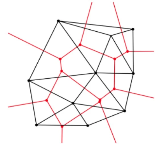
   In the future, I’ll probably make a post on Delaunay triangulations as well. Refer to the above picture for the graph dual of a Voronoi diagram.
   (The voronoi diagram is in red, the Delaunay triangulation is in black)

   Each Voronoi region has a point in the Delaunay triangulation, and these points are connected if the regions share an edge.

   Higher dimensional Delaunay “mosaics” exist as well for higher dimensional and higher order Voronoi diagrams as well, but they haven’t studied as completely as 2-dimensional order-1 diagrams.

Some Applications

There are tons of applications of Voronoi diagrams and Delaunay triangulations in fields like crystallography, but I am more interested in machine learning.

1. Simple classifiers

   For classifiers such as \(k\)-Nearest Neighbors classifiers, Voronoi diagrams show which regions sample data can be located in to categorize as certain classes.

2. HNSW

   The reason I got into this area of research was because as I was going through the HNSW paper, I noticed they make this bold assumption that slightly randomized small worlds graphs approximate Delaunay triangulations and don’t provide any backing behind it.

   Delaunay triangulation graphs have high navigability properties, ideal for graph search, which HNSW builds on in their paper. In practice, HNSW shows incredible results akin to logarithmic, as specified in the paper. But, the theoretical grounds haven’t been fully covered as far as I can tell.

The End

Thanks for reading! If you’re interested in what I’m doing, feel free to reach out and contact me!