What is FAT12? FAT12 stands for File Allocation Tables, 12. It was introduced in 1977 (almost 50 years ago!) and has many descendents, such as FAT16, FAT32, and exFAT. It’s a file system that was used in early computers, and is can likely be found on any floppy disk you come across. As the first file system that I’ve ever delved into, I can say that it’s fairly simple to learn.

Many people have tried to explain this, but in my experience, they all miss some small portion. With that in mind, let’s start learning!

Quick Overview of Storage Devices

I’d like to start off with what storage devices actually do, because I always accidentally confuse people by assuming they know this. A storage device is literally something that holds data. This can be a book, a document, a drawing, a harddrive, etc. Anything that can hold information (which is literally everything) can be a storage device. However, it’s much easier for computers to interface with storage devices that hold data in terms of 1’s and 0’s. Examples of these are: Floppy disks, Hard disks/drives, SSDs (Solid State Drives), Thumb drives (USB-flash storage), M.2 SSDs. There are countless types. However, all you really need to know about them is that they hold a sequence of 1s and 0s in a specific order, which we can change whenever we want.

Computers are made in a way such that it’s much easier to deal with 8, 16, 32, or 64 bits at a time. These are the most common, but most powers of 2 (greater than 64) are also common. A sequence of 8 bits is called a byte. The capacity of most computer-interfaceable storage devices are measured in bytes. For example, the computer you have might have 250 gigabytes of storage. As you might know already, giga means 1 billion, so you have 250 billion bytes of memory at your disposal! The prefix giga comes from the orders of magnitude prefixes for SI units, which you can find at this link.

There is also another type of prefix, which is very similar to the SI prefixes, but it’s in powers of 2. You can find a table for them here, and notice how similar they are to the SI prefixes! This is often a source of confusion. I only learned about them recently as well! So, if you ever see an ‘i’ in the middle of a byte unit, just know it’s in binary. Meaning, 1 KB = 1000 B, but 1 KiB = 1024 B. (Kilobyte vs Kibbibyte) Generally, they are very similar, so it usually doesn’t matter, but we’ll be getting into very specific amounts of bytes very soon, so it’s good to know the difference.

Partitioning

It’s kind of ambiguous when defining a partition of a disk, without using ‘operating system’, so I’ll define it in the mathematical sense. Imagine you have a set of numbers \(\{1, 2, 3, 4, 5, 6, 7, 8, 9, 10\}\). A partition of this set is a set of sets where the numbers contained in those inner sets aren’t duplicated at all, and they make up the whole original set. For example, these are partitions of our original set:

\[\{ \{1, 2\}, \{3, 4\}, \{5, 6\}, \{7, 8, 9, 10\} \} \\ \{ \{1, 10\}, \{9, 8\}, \{2, 7\}, \{3, 4\}, \{5, 6\} \} \\ \{ \{1, 2, 3, 4, 5, 6, 7, 8, 9, 10\} \}\]

And these are not partitions of our original set:

\[\{ \{1, 2\}, \{3, 4\}, \{5, 6\} \} \\ \{ \{1, 10\}, \{9, 7, 8\}, \{2, 7\}, \{3, 4\}, \{5, 2, 6\} \}\]

The first one is missing numbers \(7-10\) and the second one has an extra 7 and 2. Disk partitioning is very similar. We have a disk with x bytes on it, and we can partition it so that the first half and second half are different partitions. Notice how “partition” can be used as both a verb and a noun. Also notice how each partition (n) has no overlapping with other partitions, and the sum of all partitions makes up for the whole disk space.

For the purposes of simplicity, I won’t be using any file system partitioning, which is where partitions of the disk are used for completely different filesystems. We’ll treat the disk like it’s one big partition, and our filesystem will take up the whole partition. However, that’s not to say we won’t be using any partitioning! It’s actually very important. For example, for this specific filesystem (FAT12), we need a section which tells us which parts of the disk are free to store data in (which, by the way, is in a different section!) Also, since disk partitioning is usually associated with having a different filesystem on each partition, I’ll call them sections from now on.

Structure of FAT12

There are a couple different sections in FAT12. Here’s a list of them, in the order that they appear on the disk:

• “Reserved” Section
• File Allocation Tables (hey, that’s the name of the filesystem!)
• Root Directory
• Data Section

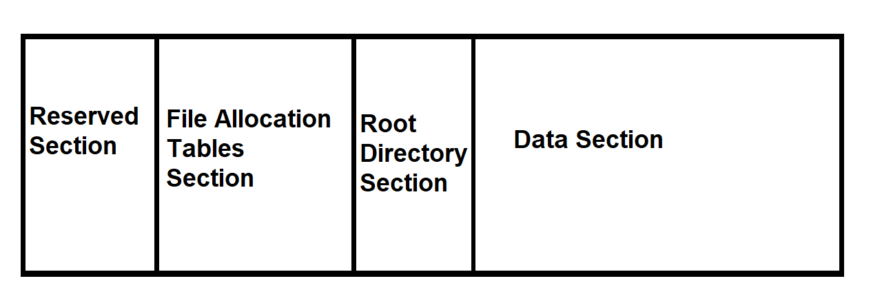
Each of these sections also is split up, but these are the basic ones that we need to remember. In FAT12, the sections are split up slightly different to how it’s split up in FAT16 and FAT32, so from now on, I will only be talking about FAT12. However, they are similar enough that later, we can use the base understanding that we are building right now to continue.

One term I need to define before we continue, is a sector. In the file system sense, a sector is 512 bytes. Apparently this is configurable, however we’re going to keep it at 512 bytes for simplicity. From now on, always assume a sector is 512 bytes. The other term I need to define is a cluster. A cluster is just a group of adjacent sectors of a specific length. Again, for simplicity, I’ll be using 1 sector per cluster, meaning our math should simplify a bit. The only place where we’d rather use clusters than sectors is in the data section, as mentioned in the list above. Let’s get into what each section actually does.

Reserved Section

The first section is only 1 sector long. Notice how it’s a sector, and not a cluster. That’s because we’re in the reserved section, not the data section. The first sector of a disk is a special sector called the “boot sector”. It contains machine code that your computer automatically loads when you turn it on, and it runs that code which is supposed to load your operating system. It’s very interesting, but it’s also a topic for another post.

One notable thing about the boot sector is a group of bytes called the “Bios Parameter Block”, or BPB for short. The parameter block is full of specifically ordered bytes in an exact length to configure things such as how big a sector is, or how many sectors long a cluster is, or how many entries can be in the root directory, etc. However, we won’t need to worry about that in this post, since 1. This is all conceptual (for now), and 2. We will define this stuff as we go.

Wow, first section out of the way! That was easy, right? As it turns out, that was the easeist one by far. Onwards!

The Data Section

I’ll explain the data section before the file allocation tables, since it’s the second easiest section to understand. The data section is, as the name suggests, the section where we store all of our data. So, if we have a text file, the actual ascii/utf-8 bytes representing the text would be stored here. If you had an image, it would also be stored here, in binary format. (That may entail each pixel being stored as a certain sequence of bits) Any file that you would have on your computer is stored in this section of the disk.

Since we have to store all of our files here, this is the biggest section, by far. According to wiki, the maximum volume size for a disk using the FAT12 system is 32 MiB. I haven’t defined what a volume is, so just understand that the maximum size of the data section can be 32 MiB minus the reserved section, minus the file allocation tables. That turns out to still be really close to 32 MiB.

You may ask, “Why would anyone want to use a file system that can only support 32 MiB? I have a single image file that’s larger than that!” I would tell you that that’s a good question! But, remember, this file system was introduced in 1977! Back then, some people thought that no one would ever need more than 640k of memory, but today, even the lowest end computers have at the very least 2 GB of memory. (Memory is not the same thing as storage, but my analogy still stands.) Later, we can upgrade to FAT16 or FAT32, which can hold more data.

One other thing to note is that directories are actually stored as files. We can explore how this works later, but just know that it’s stored as a file, containing “links” to all of the files that it contains.

The last thing you should know about the data section is that the very first file is

File Allocation Tables

The file allocation tables are what characterize this file system, and is also the hardest section to understand. This is essentially a linked list which tells us where our files are and which parts of the disk are free for us to put more data in.

If you don’t understand how linked lists work, I urge you to do some research. They are a common data structure used for making dynamically sized lists, and can be modified slightly to make trees, graphs, and even weighted trees and graphs.

Anyway, the FAT linked list is all in binary. You may be wondering how this works, and rightfully so! (It’s actually really interesting!) Essentially, each entry in the list is exactly 12 bits. (Hence the name of FAT12) We’ll think of the table as 12 bit entries for now, but when we get into how we would implement this in the real storage device, we will need to start thinking about 12 bits as 1.5 bytes. (It’s pretty icky…)

Example 1

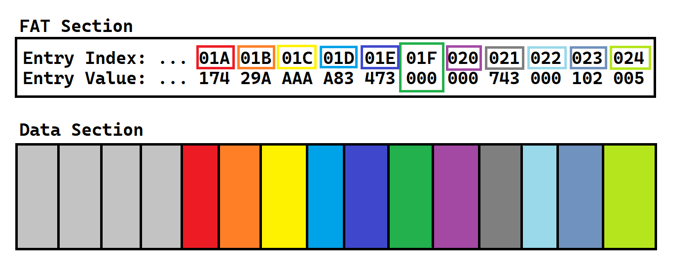
Here’s an example of how a file is stored. At first, every entry is set to 0. This is a reserved value, which means “hey computer, there’s no useful data here, so you can store whatever you want here!” It indicates free space. In order to find where on disk we should store our file, we need to find the first FAT entry that is free (AKA equal to 0)

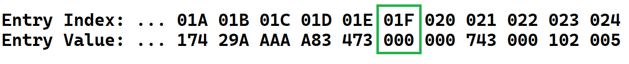
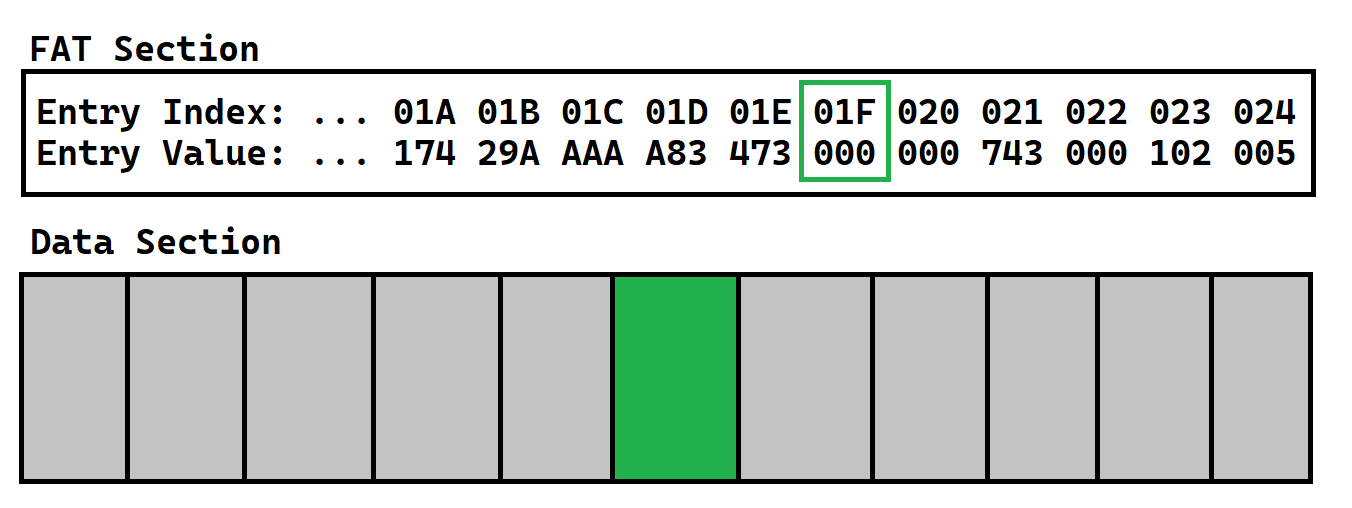
The index of this FAT entry is equal to the index of a cluster in the Data Section. This is the first cluster that we will use to store our data in.

Now, let’s imagine that our file is 100 bytes long. Since a cluster is equal to 1 sector, and a sector is equal to 512 bytes, we have plenty of space to store our file in here! So, let’s just copy the 100 bytes of our file into the cluster.

Now, our entire file is stored in the data section. However, our computer will never know that a file is stored there, since we never updated the FAT! Remember, it’s still set to 0, which means “this space is free!”

The way we assign the FAT entry is by giving it the index of the next cluster of the file. BUT, since our file only takes up 1 cluster, we don’t have anything to put here!

This is where another reserved value comes into play. A value of 0xFFF in hex will signify that this cluster is the last cluster of the file. Effectively, this signifies the EOF. (End Of File)

So, we’re done! That was pretty easy! Before I answer any other questions on how the computer may find that file, let’s try another one.

Example 2

Imagine our file is 1536 bytes long exactly. Well this is a nice number, because it’s exactly \(512 * 3\) bytes! This means that it’s exactly 3 clusters long! (Remember, 1 sector = 1 cluster = 512 bytes)

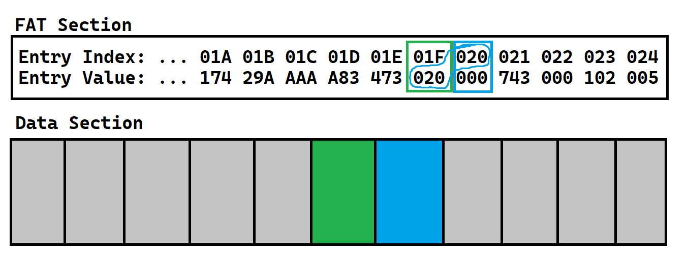
We always start with the first cluster. So, first we find the next free entry in the FAT. (Equal to 0)

Then, we get the index of that entry, and match it up with the cluster who has the same index. We store the first cluster of our data into this cluster that we just specified. Next, we would store something in the FAT entry. Remember, we store the index of the *next* entry in the FAT. But, seeing as we don’t have a next entry yet, let’s keep this current one in mind and move on.

Now, we need to store the next cluster of our data. Let’s find a new free FAT entry.

Now, let’s find the cluster with the same index of that entry!

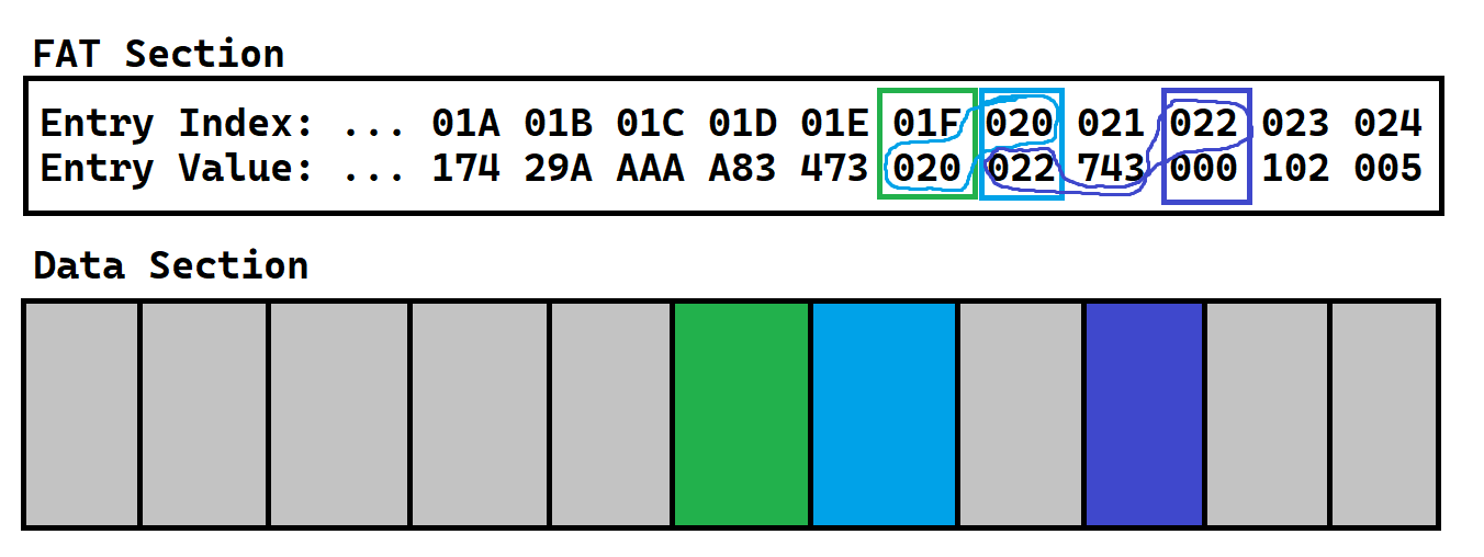
Now, we can store the next cluster of our file in here. That would be bytes 513-1024, since bytes 0-512 are stored in the first cluster we had. And next, we need to fill up the FAT. Think back to last time: we now have that “next entry” ready! That “next entry” will just be the index of the current cluster we’re on.

So, let’s go back to the old index. Last time, we wanted to store the next index, but we didn’t get it yet, but now we have it! So, let’s store the current index in the old index.

Phew, that was a lot of emphasized text! But, we aren’t done! That was only 2 clusters of the 3 that our file requires. Remember, it was 3 clusters long.

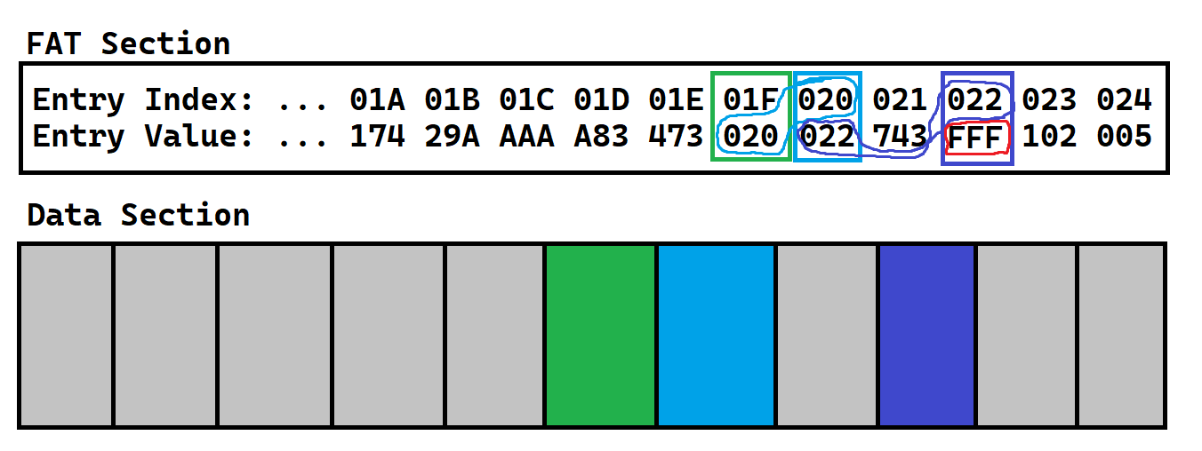
So, let’s find the next free FAT entry. Then, let’s find the cluster with the same index as that FAT entry. Now, let’s store bytes 1025-1536 (the 3rd cluster) in there. That’s the last of our data! Last, don’t forget to update the FAT table! So, let’s store the current index in the old index.

And finally, since this is the last cluster of the file, let’s store the special reserved EOF value in the current index.

To Generalize

That’s probably the most confusing part of FAT. If you got lost, I encourage you to read that second example again, and definitely look at the pictures for guidance. We can be generalize this method in a small algorithm.

For each cluster in the file we want to store:

1. Get the first free/empty FAT entry
2. Store the current file cluster in the cluster at the index of current FAT entry
3. Set current FAT entry to EOF (0xFFF)
4. Set previous FAT entry to index of current FAT entry (if there is a previous FAT entry)

Notice how I made step 3 set the current entry to EOF. This is actually a small shortcut that I just thought of, which makes it so that we don’t have to check if the current cluster is the last cluster in the file, and also allows us to simplify our find first free entry algorithm. If you think about it, when we are finding the next free entry, in the examples above, the last entry is also set to 0, so we have to purposefully skip that one. If we set it to an EOF, we won’t have to take that into mind.

Reading a File

Now, let’s try reading a file given the index of the first cluster.

Well, we know that the index of the cluster is attached to the index of the FAT entry, so let’s get that FAT entry. We also know that each FAT entry will point to the index of the next FAT entry for the file, which also is the index of the next cluster. When we come across a FAT entry that is equal to 0xFFF, we know that’s the end of the file, so we can copy the current cluster and end the search.

To Generalize:

Until we reach an EOF entry:

1. Copy the cluster at the index of the current FAT entry into memory
2. Set the current FAT entry to the one stored in the current FAT entry

Simple! I don’t know much about other filesystems, but even if I did, this would probably seem very easy.

Directories

Think about this from a larger standpoint. When we turn on our computer, how does it know which code to run? Well, we’d determine that if we were writing the bootloader. (Remember I mentioned that earlier for the reserved section?) We’d want a system of easily grouping files for easy access and organization. This is exactly what directories are for!

Let’s talk about directories for a second. As you may know already, a directory is like a manilla folder, if files were paper documents. It’s just a way to group files. In the FAT systems, directories are actually stored as files! This makes it a lot less complicated and more generalized. So, to read the file and find all of the clusters in the file, we’d read the FAT table exactly the same way for any other file.

Imagine we performed the file read method on a directory. Now that we have the directory in memory, how do we find the files inside? Well, the directory file is just full of 32 byte directory entries. If you have experience with pointers in C, each directory entry is like a pointer to the file, along with attributes. Every byte of the 32 bytes is used for something, including the filename, file extension, attributes, timestamps, the first cluster of the file, file size, and if this entry is actually a subdirectory file. If you want to see exactly which bytes are used for what, I recommend you look at page 5 of this document. In fact, read the whole thing! It was one of the documents I used to learn FAT12.

One thing I noticed, which was kind of funny, was that the file size is 32 bits long. That means, it’s possible to have 4 GB files in FAT12, even though the entire file system can’t be larger than 32 MB! In FAT32, the max file size is 4 GB, so eventually we can take advantage of all of those bits.

Anyway

To get all the files in a directory, we split it into 32 bit directory entries. The file name is the first 11 bytes, and the first cluster of the file is in bytes 26-27. Notice the first cluster is 2 bytes long, even though FAT entries are only 1.5 bytes long. In FAT12, the last 4 bits of those 2 bytes are just never used. So, to get a file by name, we can compare the first 11 bytes of each entry to the name we are looking for. If the names match, we can load the file using the first cluster in bytes 26-27. Also very simple!

The Root Directory

Generally, the root directory is 14 sectors long. Again, this is configurable in the BPB (Bios Parameter Block), but for the purposes of convention, we’ll keep it at 14. Since each directory entry is 32 bytes long, and each sector is 512 bytes long, there can be 16 entries per sector. The root directory has 14 sectors * 16 entries per sector, which is 224 entries.

Notice how I was talking in terms of sectors and not clusters. This is because in FAT12, the root directory is kind of awkward. It’s not actually in the data section. It’s located right after the FAT section, and right before the data section.

So, as you can see, reading the root directory will be slightly different than reading any other directory. In reality, getting stuff from the root directory is actually slightly easier. For one, it’s always 14 sectors long, and it’s always in a specific location (right after the FAT section), so there’s no need to read the FAT table. But, since it’s not in the data section, we’ll need to calculate the sector number slightly differently. (We’d just not add the 14 sectors in the root directory, like we would for the data section, since it’s located after the root directory.)

Having a root directory in a constant place allows us to structure all of our files in a consistantly locatable tree. What I mean by this, is that we can make subdirectories in the root directory and store files in there, which emulates a tree structure. This allows us to traverse the tree to find a file at a specific path! That’s useful for loading system code files into memory to run, which will allow us to build even more tools to explore the files.

The End

That’s essentially all you need to know to get started on building your own FAT12 implementation. Obviously, that’s not all there is to know about FAT12. There are plenty of limitations that I haven’t discussed. I also didn’t discuss many of the file attributes, many of which can be considered as important. I’ll likely make more in-depth posts about more specific parts of the FAT12 system in the future.

If you’re interested, I’m making a FAT12 implementation in rust right now. I’m using it as a project to both improve at rust and FAT12. It’s a shell that you can copy files from the host OS to a FAT12 disk image, which I can then use to run on a VM emulator. If you are interested in it’s progress, you can check out its GitHub page here, and you can watch my occasional streams on twitch

If you spotted an error in this post, or have something that you’d like to add, please make a github issue or pull request, as linked to in the footer.

Thanks for reading!