Basic Introduction to Generative Adversarial Networks (GANs)
2021-08-01
What is a neural network? You may have heard of neural networks before, and you may know that they mimic brains. Many people’s knowledge on neural networks falters after that. However, I’m here to provide a basic overview of what they are, and how they work.
A Neural Network, (or NN for short) is a model of how a brain could theoretically work. I say model, because NNs are just complex structures made out of a bunch of tiny little parts. In a real brain, these parts would be the neurons, and scientists have decided to name it the same thing in our model. A NN is just a bunch of neurons connected to eachother.
Now, being modeled on the computer and restrained by the digital nature of silicon logic, it would take a lot of computation to simulate the exact voltages being pulsed through each neuron. So, scientists have simplified it down to a bunch of linear equations, generally represented by vectors and matrices, carried out through dot products.
Why are we able to make approximations of neurons using linear algebra? Well, consider the structure of neurons in a real, human brain.
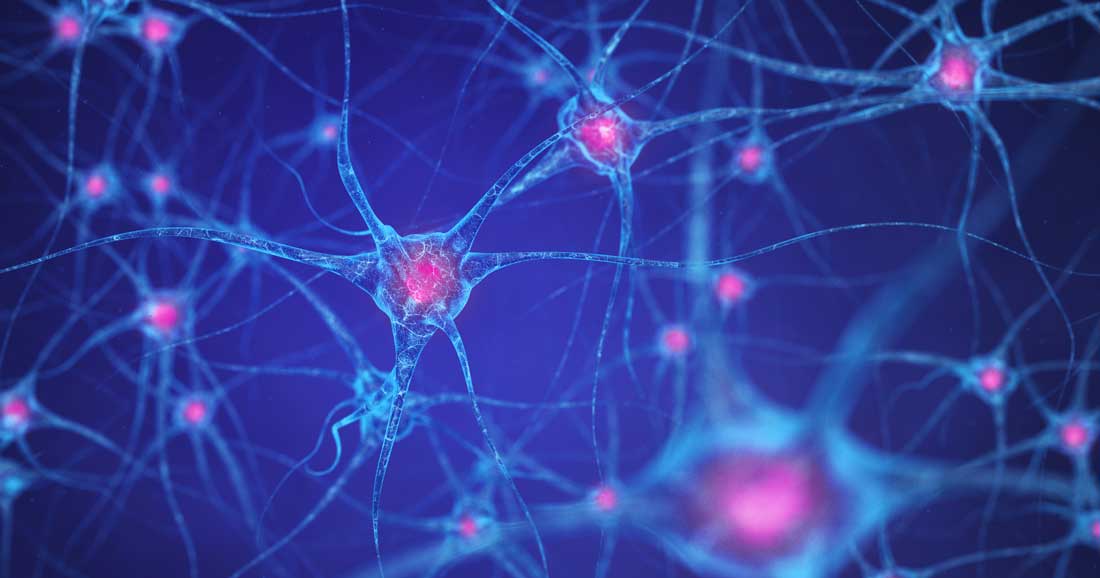
Here, you can see how each neuron is connected to many other neurons, with varying connection “intensities”. We can make our own model with similar properties, which can be visualized as the following.
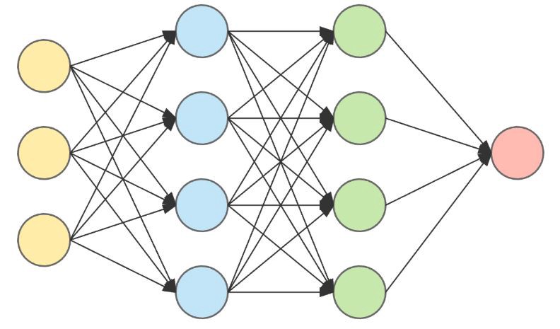
Notice the similar properties here.
- Each neuron is connected to a number of other neurons.
- Each connection has a certain “intensity” or “weight”. (Can also be thought of as length)
Also, notice some other properties.
- Information/voltages/signals from each neuron only flows from left to right.
- There are input neurons. (Yellow)
- There are output neurons. (Red)
- The neurons in vertical columns can be grouped together and called “layers”, representing each “step” of getting an output.
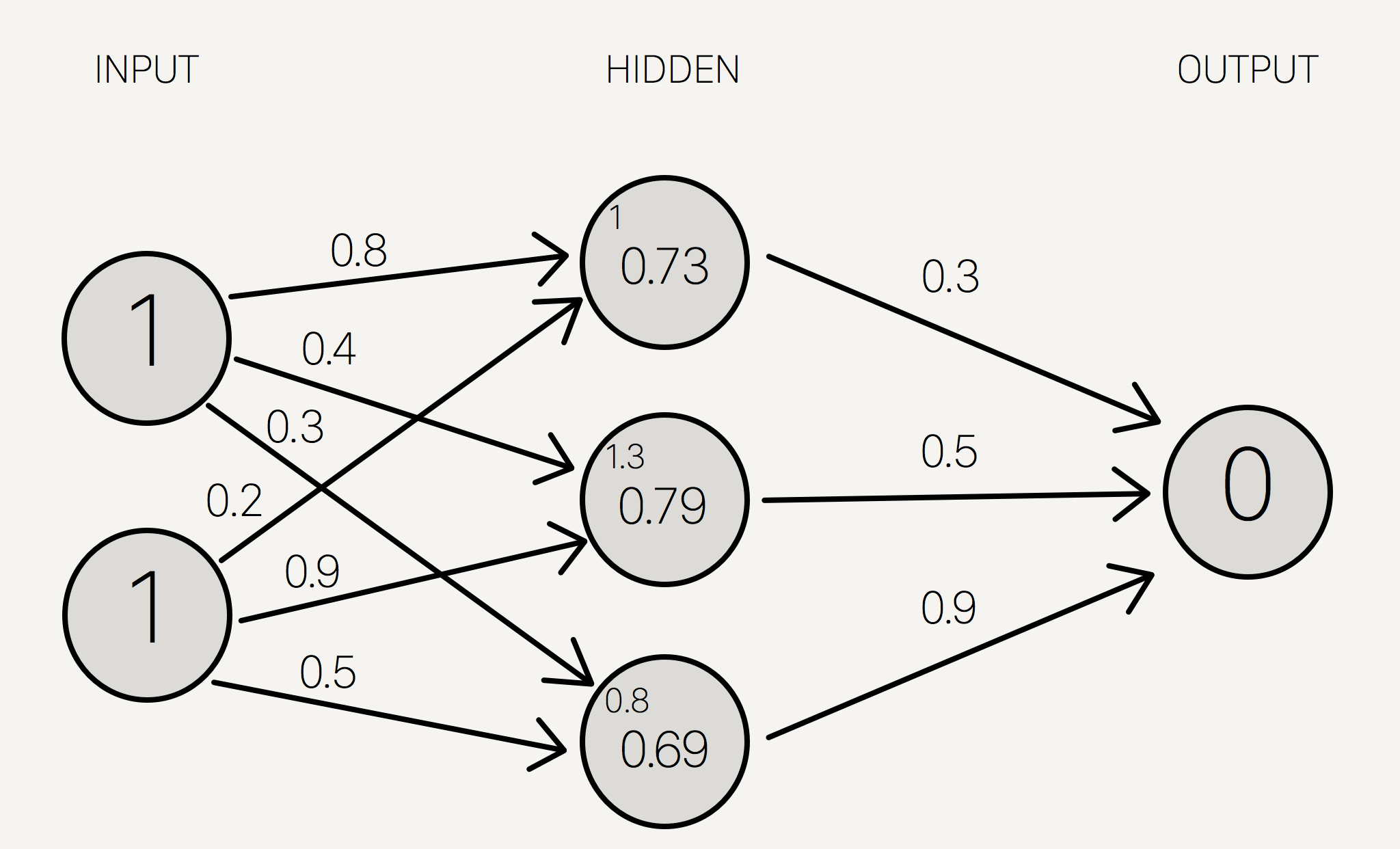
In a normal human brain with relatively unstructured neurons, we wouldn’t know where the network starts or ends! However, modeling a network like this makes it much easier to find definite inputs and outputs, much less calculate outputs from certain inputs. So, how can we calculate some outputs? First, take some inputs, as a vector to represent each voltage level in the input layer. Each connection/edge has a weight/intensity, so how can we represent the voltage encountering such resistance? We can multiply the voltage by the edge weight. This effectively represents the lessened/heightened voltage due to the connection strength.
Once we get all the voltages at the end of each connection, we need a way to combine them as input to the next node. The easiest way to do that is just to get the arithmetic sum. Now, we have the voltages of the first layer. Hooray! In order to keep going, we repeat the process.
- Multiply the input values by the edge weights.
- Add them up, and set the sum as the inputs to the next neuron.
It’s that simple! One who is familiar with linear algebra may recognize the act of adding a bunch of products. That’s right; we can do this all with matrices, dot products, and matrix multiplication! We have a vector of all the neuron inputs. The weights corresponding to each output neuron can be put into a matrix, where every row corresponds to a different input neuron, and every column corresponds to a different output neuron. Multiplying these two matrices will multiply each input value with each edge weight, sum them up nicely, and store it in a vector. Linear algebra basically just served us neural networks on a silver platter!
Training a Neural Network
This topic is much more complex, and could be put in its own blog post. However, to get the gist of it:
We first have to have a bunch of data to train the network with. That could be the color values of each pixel in an image, amounts of ingredients in certain cookies, survival statistics on the Titanic incident, etc. We start out with a neural network with a bunch of random edge weights. When we give it some inputs and calculate the output, the neural network will give us some weird random answer, due to all the random numbers in the weights. In order for the network to give us sensible answers, we need to adjust each edge weight until the outputs become reasonable. We can’t do this manually, though.
So, we have a predicted output (from the neural network) and an actual output, from our dataset. Given a theoretical value and an actual value, it’s trivial to calculate the percent error. Obviously, we will want to minimize this error, because we want the neural network to give answers that represent real answers.
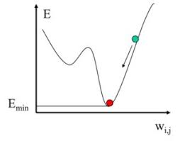
We adjust the weights of each neuron. Our goal is to adjust each weight by minimizing the error of the entire network. This can be done by adjusting each weight individually by a small amount and calculating the error for each adjustment. Then, using basic calculus, we can use a central difference approximation to approximate the derivative of the error with respect to that edge. From there, we can just adjust the weight to minimize the squared error, using the derivative approximation.
Then, we just do that for each edge, et voila! We are left with a network that has slightly less error than before.
What is Deep Learning?
‘Deep Learning’ is a term that is often thrown around for many different machine learning models. A combination of its denotation and some theory behind neural networks will be sufficient to understand its meaning.
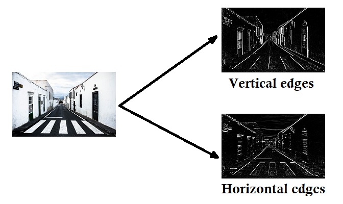
Each layer in a neural network is a way for our model to recognize different patterns. The first layer would be able to recognize simple patterns. For example, it could recognize if two inputs were on at the same time, and output that. This could be like an AND gate. If we were using images, one node in the first layer may detect a vertical edge with black on the left side. It could also detect vertical edges with black on the right side, horizontal edges, edges with different colors, and even dots or circles.
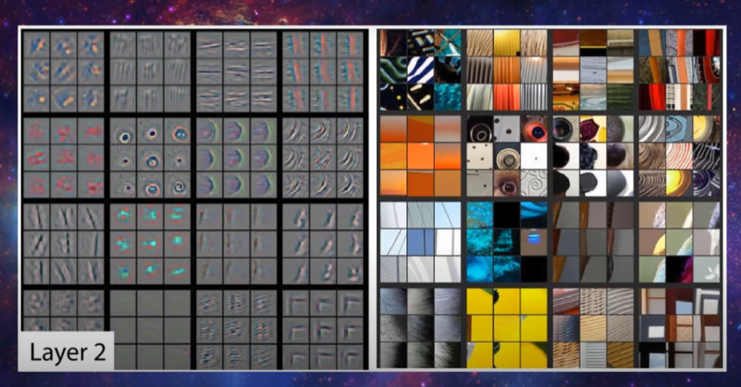
Moving on to the second layer, we can use the simple patterns in the first layer to detect slightly more complex patterns. For example, the network could combine multiple edges to detect a corner. It could also detect parallel edges, which would signify a line. Using extra edges and dots, it could detect a larger circle.
For the third layer, the network could detect more complex patterns, like an actual eye or mouth. Then, the fourth layer could detect a whole face, and the fifth layer may be able to detect a whole person.
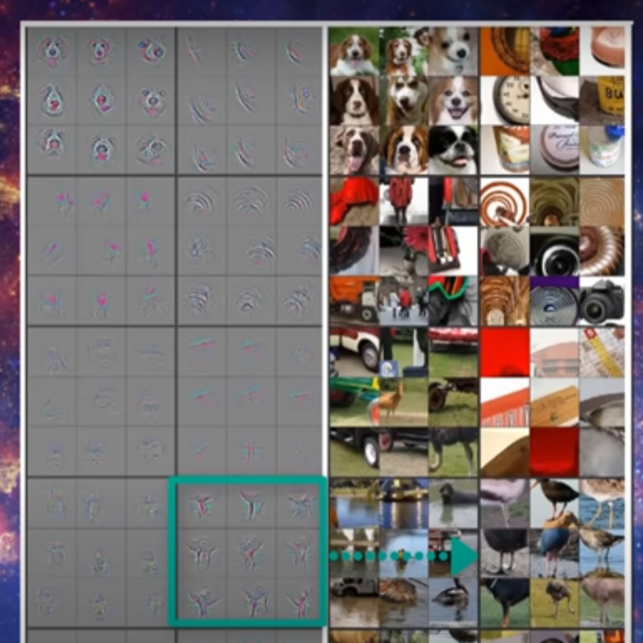
As you can see, the more layers a neural network has, the more complex patterns it can actually detect. When a network has the property of having a lot of layers, it is able to make more complex and deep connections within the dataset that it is given. Hence, deep learning.
In basic terms, deep learning just means the network has many layers, or capacity for complexity.
The network I just described is definitely possible, but there are a few things one should note. The first thing is that you don’t actually define each node as being able to “recognize” certain patterns, like edges, corners, eyes, or people. When you train the network, it alters itself to be able to detect certain patterns. Obviously, the stated patterns are possibilities. However, trained neural networks tend to be convoluded. They usually develop their own patterns, like maybe if a couple strange colors are near eachother.
Using traditional methods of training, as explained above, it wouldn’t be possible to set the patterns that the network understands. Instead, it chooses its own patterns, through it adjusting its edge weights by minimizing error.
The second thing we should note, is that I described a convolutional neural network. Normal neural networks would have to be able to recognize a pattern on every single combination of pixels, which would take a lot more neurons per layer. However, convolutional neural networks are able to use a cool trick to recognize patterns anywhere.
Convolutional Neural Networks (CNNs)
The main difference between a convolutional neural network and a normal neural network is the convolutional layers. This is where a filter is created, and convolved around the image.
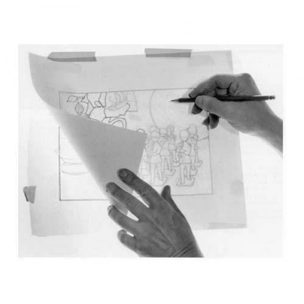
A filter can be thought of as transparent tracing paper. It contains pixel values, like an image, but it’s main purpose isn’t to be observed, rather, to be compared.
Imagine our input is the rgb values for each pixel in an image.
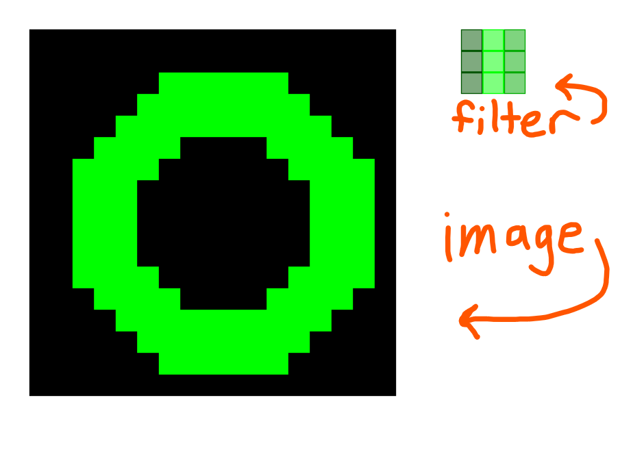
Speaking at a high level, the filter is first compared with the top left corner of the image. The pixels in the image will most likely have a different color than those in the filter, so we calculate an error value. This error value is then stored in the top left corner of a new image. This new image in reality is just a vector of numbers, but we represent it as an image to show where each number comes from.
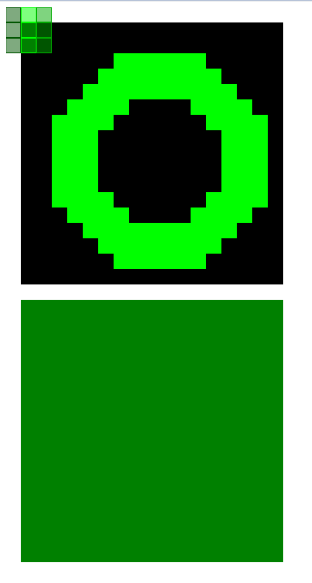
Then, we move the filter over by 1 pixel, which is called a stride. And, rinse and repeat.
- Calculate the error
- Store the error in the corresponding square in a new image
- Move the filter to the right. (If at the end of a row, move to the beginning of the next row.)
The process of comparing the filter with each section of the image is called convolution.
At the end, we are left with a little image, full of error values. The parts with the least error tell us where the filter matched the image the most, and the parts with the most error tell us where the filter matched the least.
Just like any other layer, convolutional layers have inputs and outputs. The input is the initial image, and the output is the image filled with the convolving error data.
Generally, there are only a couple convolutional layers per CNN because they take so much more time to compute. Plus, once the general patterns are detected, normal neural network layers are able to put two and two together to predict what’s in the image. For example, if the convolutional layers determined that there was a dog face, a human face, and a long line in the image, the neural network could determine that the image probably depicts a human walking a dog on a leash.

Generative Networks
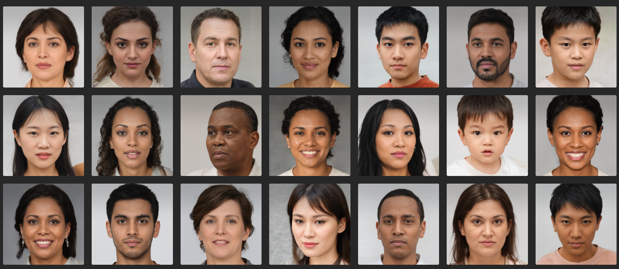
You may have seen images of human faces that don’t exist, but instead were generated by a computer. Those were created using generative networks.
As you know, neural networks have a bunch of input and output values. We’ve discussed models where the input layer holds an image, but what about the output? There’s nothing stopping us from making a large output! (Make sure to also consider other things, like ingredients for a certain recipe, or health statistics for a certain person with a disease)
That’s exactly what a generative network is; a neural network that has a bunch of outputs, possibly to be represented a different way. (An image, for example.) Now, it’s common that these generative networks have a bunch of inputs as well. Let’s think about the theory; if there were only a small amount of inputs, the model wouldn’t be able to generate a large variety of outputs. Instead, it would be restricted to certain images due to a lack of variety in the inputs. However, if we had a ton of inputs, we would have to blame the lack of variety on the edge weights inside the network, which would just come down to training.
The set of all input vectors for such generative networks is called the latent space, which has many interesting properties that I won’t be getting into today. Maybe in the future, though.
CNNs as Generative Networks
There are many, many different types of generative networks, but the one that I’ll be going into are the generative convolutional networks.
The theory is pretty simple, actually. We just treat the input from the latent space as some type of image, itself. Then, we can use convolutional layers to not only find and relate certain patterns in the latent space, but also to give different numbers of outputs until we reach the desired image size.
For example, imagine the latent space has 100 dimensions, and we want our output image to be 20x20 pixels large. We could have a convolutional layer that detects patterns in the latent space, then feeds the output into another layer called a reverse pooling layer. All you need to know about this layer is that it basically just scales up the image.
Using multiple convolutional layers and upscaling layers, you can eventually land at an output vector size of 400, aka 20x20.
Discriminator Networks
A Discriminator is an essential part of a GAN. It’s basically a network that takes an image as an input, and has a single output, which is the probability that the image is real or not. For a basic understanding, that’s all you need to know!
CNNs as Discriminator Networks
It’s a good idea to use convolutional layers in discriminator networks. Since it’s the discriminator’s job to figure out if the image is real or fake, it needs to be really good at recognizing certain things in the given image. Luckily, convolutional layers are great at that! They help networks recognize patterns.
Convolutional layers allow the discriminator networks to predict with more accuracy and less training, due to the pattern-recognition nature of convolution.
Duality
Finally, we get to understand what a GAN is, as a whole! GAN stands for Generative Adversarial Network. We know what a generative network is, so that’s easy to understand. The adversarial part is the part that makes GANs so revolutional, though.
As you may know, an adversary is like an opponent. The first thing that may come to your mind about a GAN is a network fighting an adversary. A strange thought, but one that holds truth nonetheless. In the case of a GAN, the adversary is actually a second neural network.
A good analogy of a GAN is like an art forger, and an art critic. It’s the art forger’s job to make art that looks like it’s real, so they can sell it and get rich (or something). The art critic’s job is to look at a piece of art, and figure out if it is genuine/authentic, or if it has been forged. The forger and critic have varying levels of accuracy, though.
At the beginning, the forger may make paintings that look like complete garbage. Obviously, the critic would have an easy time figuring out that it was forged. But over time, the forger would improve with both feedback from the critic and time spent studying authentic images to imitate them.
Eventually, the forger will become good enough to fool the critic into thinking the fake art was real. However, after a long hard search, the art critic is able to find a bunch of work by the forger. After studying said work, the critic is able to distinguish forged artwork from authentic once again!
And the cycle continues. The forger keeps improving its forging skills while the critic keeps improving its detection skills. After a while, what we are left with is a very skilled forger and a very skilled critic. So, if you wanted to buy artwork from a certain artist, but you don’t have the money for it, you could just ask the forger for some!
This is the basic idea behind GANs. The art forger is the generative network, and the art critic is the adversarial network (aka discriminator). We train the generative network using the discriminator’s output (probability of being generated) as an accuracy function. We then train the discriminator by feeding it real images from the dataset (which are classified as real) and fake images from the generator (which are classified as fake). After many iterations (aka generations/epochs) of training both networks, we should be left with a generative network that is able to somewhat replicate images from our dataset, but they are completely new.
Of course, don’t forget that the dataset doesn’t have to contain images. It can contain any type of data we want. Images, 3d models, recipes, medical data, text, audio, etc.
Why GANs are so Powerful
The fact that GANs have two different networks both competing against each other and learning from each other at the same time is what makes them so powerful. If there wasn’t another network to test the accuracy of the other, we would have to rely on only the given dataset for that. That means, we would need a larger dataset, possibly orders of magnitude larger, to get similar results. Since there’s a larger dataset to train on, that also means that we would need more computing time.
Real World Examples of GANs
GANs are so revolutionary that large companies have started testing with them.
NVidia, being a GPU designer, has worked a lot with machine learning algorithms to speed them up. They are able to generate faces that no one has ever seen before, using GANs.
Google made a machine learning library for easy implementation of GANs. They call it TensorFlow, and with it comes some of the best resources for actually learning machine learning without learning all of the theory: the documentation!
There was a series of youtube videos that actually made me aware of machine learning by a guy named Cary Huang.
Another more interactive example is this online face generator. They even reference NVidia’s paper on GANs!
Of course, there are countless other examples in the real world. You can find those that aren’t listed by just searching interactive GAN (or something).
The End
I’m learning about GANs because I plan on using them for a project, which involves generating 3d models using them. Of course, this means that I’m also a beginner (as of right now) so I may come back to this post and change some things once I know better. But, I think this post serves as a good introduction to what the theory behind a GAN is. Anyway, thanks for reading!