Long story short: if you want to see the end product, then click on the following link:

https://oriont.net/newtonfractal

In the Beginning

A long time ago, I made a newton fractal simulator using javascript with p5.js. It worked, but it was sloooooow. You can find it at this link to see for yourself.

I used all the same methods I used in this new version, except the technologies I use are different, which sped up the program a LOT.

What’s Newton’s Method?

Newton’s method is a way of approximating the roots of a function. For example, given the function \(f(x) = x^2 - 1\), the seasoned mathmatician would be able to tell you that the roots are \(1\) and \(-1\). They’d be correct, but how did they get there?

Well, simple. You could just factor it out into \((x-1)(x+1)\) and use the roots of each factor, or you could use the quadratic formula, etc. However, what if you can’t find the roots so easily, like \(f(x) = x^7 + 5x^4 + 3x - 1\)? In this case, you would use the Newton-Raphson method, also known as just “Newton’s method.”

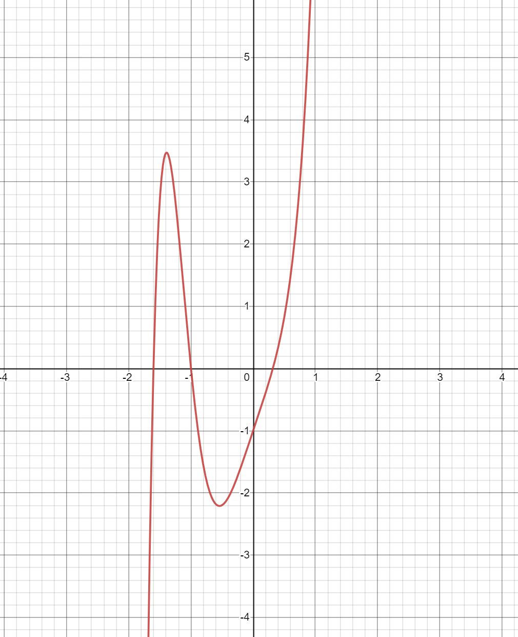
First, let’s take a look at the graph of \(f(x)\). Let’s take a random point on the graph, say, \((0.837, 4.253)\). Taking the derivative at that point will yield:

Now, how can we get to the closest zero from here? Using deductive reasoning, one can infer that if the slope is positive, then the root must reside at a lower value of x, and if the slope is negative, it must be at a higher x.

What do I mean by this? Well, take a look at the following graph, which has 3 real zeros:

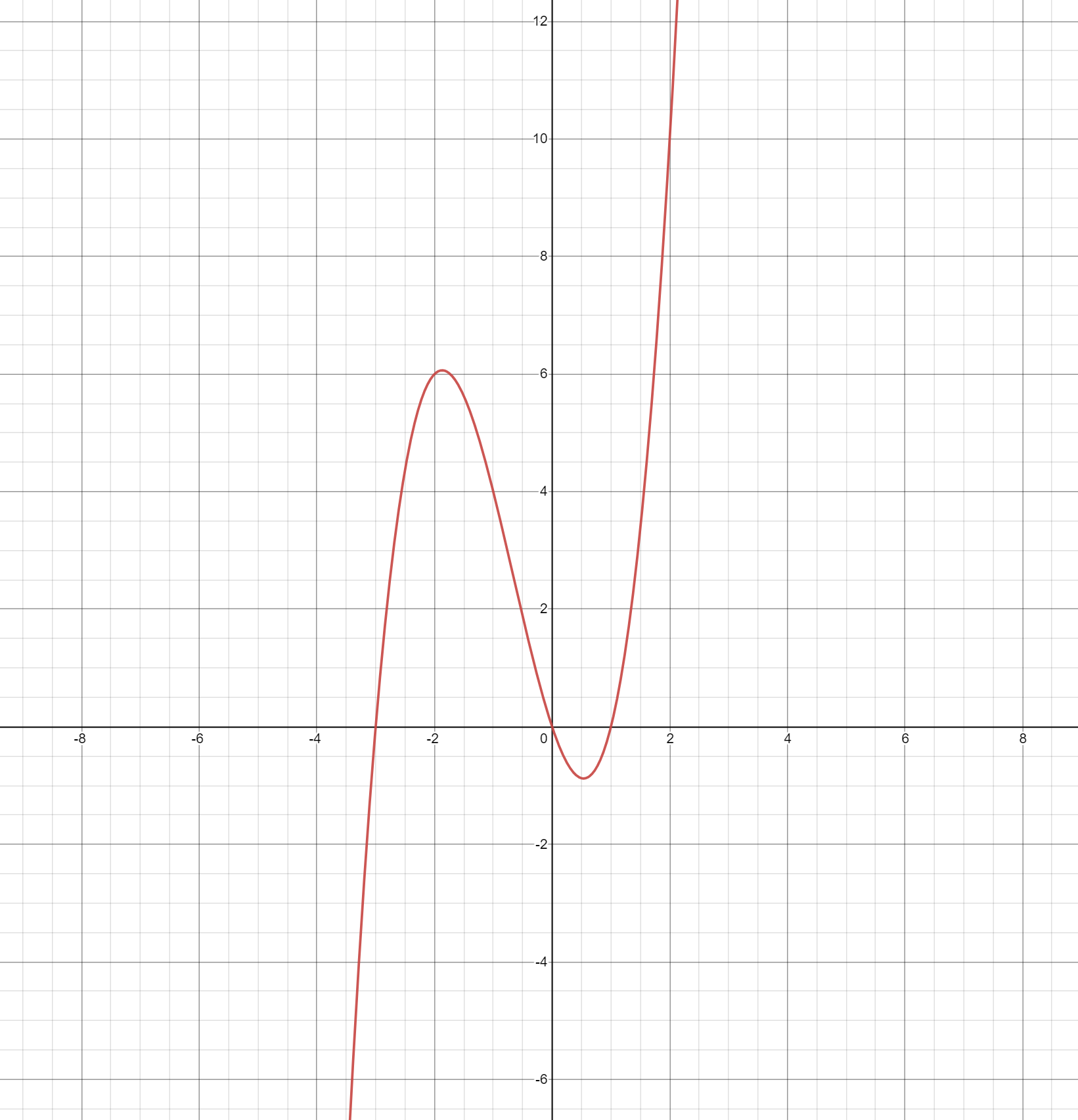
Now, take any arbitrary point (the further away from for the local minima/maxima, the better. I’ll get to that in a bit.) Now, visualize the tangent line of that point. That tangent line will have a positive slope (pointing up-right) or a negative slope (pointing down-left). Now, take a look at the closest zero. You might notice, that usually, the zero of the tangent line is closer to the actual zero, than \((x, 0)\), (x being the x coordinate of your arbitrary point). Why is this?

Well, it’s because the tangent line can be thought as an approximation of the complicated line. When we are talking about approximations, pretty much anything can be an approximation of pretty much anything else. (That’s not to say that they are good approximations). We can treat it as an approximation because it has a zero, which is what we’re looking for.

Now, this approximation (tangent) line that we have, will give us our approximated zero! Since the equation of the tangent line can be modeled (in point-slope form) as:

\(y - f(x_1) = m (x - x_1)\),

Where \((x_1, f(x_1))\) is the point of intersection, and \(m\) is the slope (aka derivative) of the line, we can model the actual tangent line as:

Now, let’s solve for the y intercept. The y intercept is a point on the line where \(y=0\), so we can set \(y=0\) and solve for x. We don’t set \(f(x_1)\) to zero, because that’s the thing we’re trying to get closer to zero! (If we could just set \(f(x_1)\) to zero, it’d be the same as finding the actual zeros, meaning we go back to the quartic functions or mega factoring or some other method.)

We have:

Now, we have an approximation for the y-intercept! It’s modeled as:

Coming from \((x, y)\), where \(x\) is what we just derived, and \(y=0\), which was the assumption that we made in order to derive it.

Now what? We have an approximation of the y-intercept, but what if it’s bad? What if we want to make it slightly better? Let’s use this method again, but in order for the next approximation to be better, we need to make sure that the initial point we choose is closer than the last one. From the first approximation, we got a point closer to the y-intercept than our initial point, so let’s use that as a starting point.

First, let’s make an equation for the y-intercept approximation, since we’re going to be reusing it.

I use the expression we got as the y-intercept approximation, except instead of \(x_1\), I use \(x_n\), since we are performing this operation more than once. And I set it equal to \(x_{n+1}\) since it’ll be used to make the next approximation.

To get the starting point, let’s use the x value as the approximation, which then allows us to get the y value using \(f(x)\). So, our next starting point is: \((x_2, f(x_1))\). Running the whole approximation process again, we get:

Where \(x_3\) is the new approximated y-intercept, calculated using \(x_{n+1}\), or in this case, \(x_{2+1}\). You might be able to see where this is going. Doing this process infinitely many times will theoretically give you the correct y-intercept for a function! But, it can only give one y-intercept at a time.

Notice, if you start at a different point on the graph, the process might converge on a different y-intercept. This is because the tangent line is closer to another y-intercept than the first one.

To give it a formal definition, let \(f(x)\) be a differentiable function, and \((x_0, f(x_0))\) is an arbitrary starting point. Use the following function:

to approximate a root. Higher values of \(n\) will yield better approximations of the root.

When Newton’s Method Fails

Earlier, I mentioned that you shouldn’t choose a point close to the local minima/maxima. Let’s try it out to see what I mean. Take a point right next to the critical point, and let’s make an approximation. I’ll just do it visually:

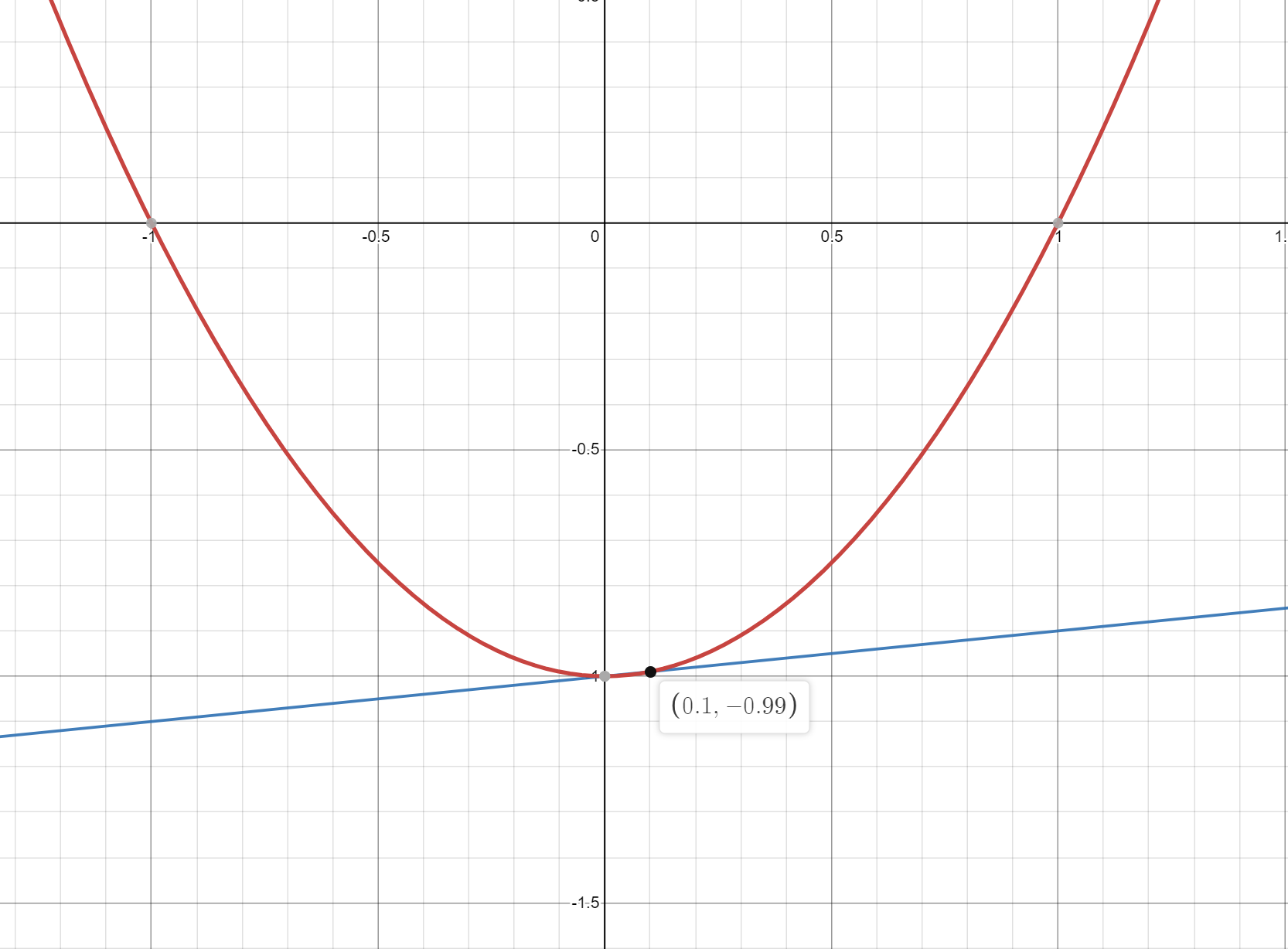
You’ll notice, the tangent line is almost horizontal, meaning the y-intercept’s magnitude is going to be very large. Obviously, this y-intercept is going to yield a much worse approximation than the beginning. However, with this function, if we continue using newton’s method, we are actually able to redeem ourselves with an okay approximation soon enough.

If we were to start on the critical point, however, newton’s method would diverge. This is because the slope is 0, meaning the next point would be:

This is one example of newton’s method diverging.

Some functions aren’t friendly with newton’s method. Take, for example,

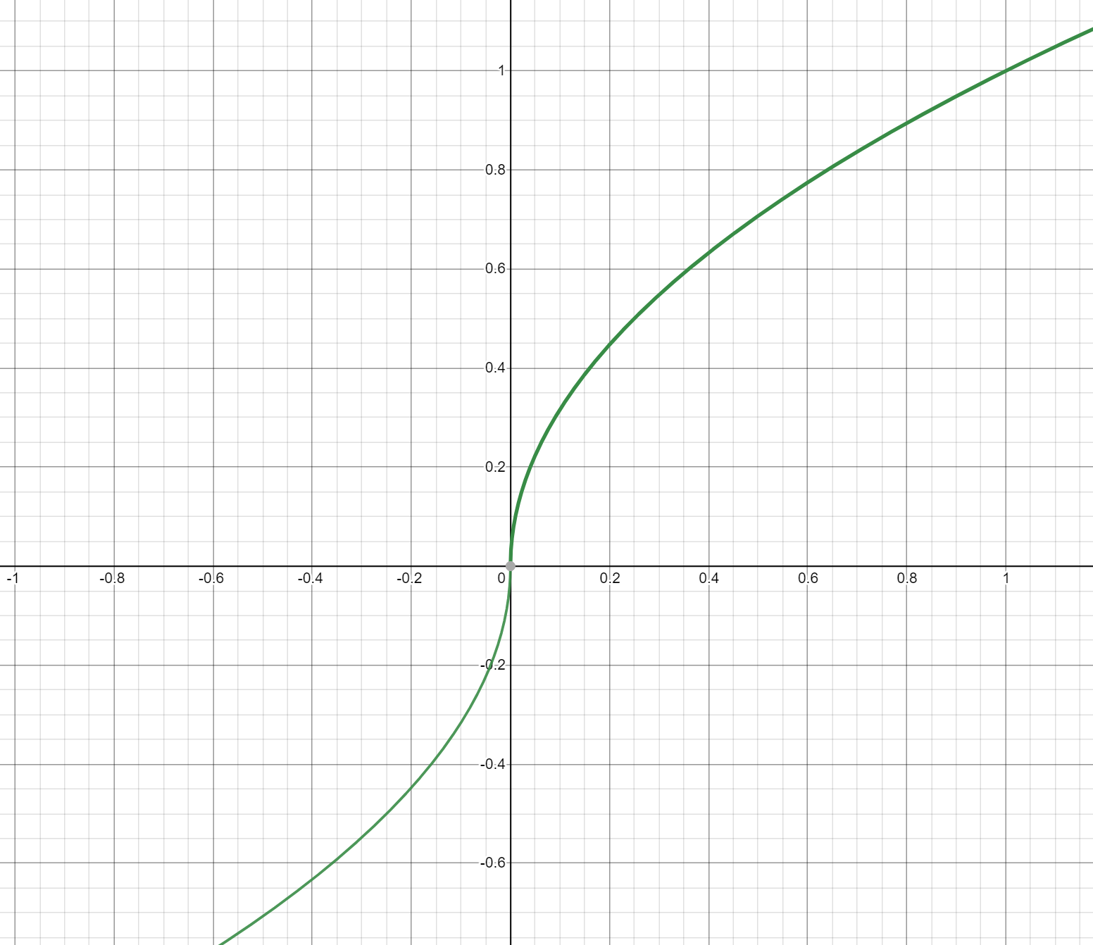
Using newton’s method on this function, starting at any point except for the y intercept, will always diverge. You would have to use a different method to approximate the roots.

Applications of Newton’s Method

• Approximating Non-linear functions

As the example above showed, what if you want to calculate the roots of a really gnarly function, such as \(y = x^10 + x^9 + x^8 + x^7 + 3x^6 + 3x^5 + x^4 - x^3 + 3x^2 - 8x + 1\)? You could either spend a bunch of time finding factors, or just use newton’s method.

• Optimization

In calculus, optimization problems are when you want to find critical points of a function. The derivatives/slopes at critical points are going to be 0, so you could use newton’s method on the derivative, in order to find said points.

• Cool fractals

This is what we’ll be exploring more today. It turns out that newton’s method works with complex numbers as well, so functions \(f(z)\) can be used to approximate zeros. Interestingly, newton’s method tends to jump around when working with complex numbers, due to the fact that certain operations with with imaginary numbers (i.e. squaring) will produce real numbers, and real numbers can become complex (through \(\sqrt{-x}\)). This means certain groups of points will converge to certain roots using newton’s method, and other groups will converge to other roots. This is what makes for a cool fractal effect.

Writing Newton’s Method in Code

Let’s really quickly go over how we could go about writing newton’s method in code. We know how the math works, so now all we have to do is create a function.

The inputs should include: \(f\), \(f'\), \(x_0\), and the amount of steps we should take. This ‘steps’ input is actually just the value of \(n\) we would like our code to stop at, since it could keep going forever. Usually, 25-50 gives pretty good approximations. Right now, it looks like this:

function newtonsMethod(f, fp, x0, steps) {
  // Code goes here!
}

Now, we have to repeatedly apply newton’s method to the variable \(x_n\), steps amount of times. We can use a simple for loop for that. Then, we just return \(x_n\). Our function now looks like this:

function newtonsMethod(f, fp, x0, steps) {
  let xn = x0;
  for (let n = 0; n < steps; n++) {
    xn -= f(xn)/fp(xn);

    // This is short for:
    // let xn1 = xn - (f(xn)/fp(xn));
    // xn = xn1;
  }
  return xn;
}

We now have a simple function for approximating the zeros of a function, given that function, its derivative, a starting point, and an approximation depth (steps). Now, let’s try it out!

As stated at the beginning of the post, the zeros for the function \(f(x) = x^2 - 1\) are: \(x = \pm 1\). Let’s see if our newton’s method function can calculate the zeros. We’ll set the starting point as, say \(x_0=15\). Note: we won’t set \(x_0\) to 0, because that’s a critical point of \(f\), and as explained earlier, it will diverge. We’ll also just use 10 steps, since it should converge pretty quickly.

console.log("Output:",
  newtonsMethod(
    x => x**2 - 1,
    x => 2*x,
    15,
    10
  )
)

Another note: for those less experienced in javascript, the first 2 arguments are lambda functions, which allow you to easily define a function with minimal code. x => means that it’s a lambda function, and it should take x as an argument. x**2 - 1 just means \(x^2 - 1\), since javascript reserved the carat (^) for the bitwise xor operation.

I added a debug log to the newtonsMethod function, showing what the value of xn was for each iteration. Here’s the output:

15
7.533333333333333
3.833038348082596
2.0469639947277685
1.267746186322663
1.028273806328014
1.0003887136477436
1.0000000755197944
1.0000000000000029
1
Output: 1

So, after 10 steps, our function gets so close to 1 that whatever precision javascript used to store the number became too low! Now, this is a very simple function so usually you want to use somewhere in the range of 20-50 steps, but for the purposes of demonstration, this should be fine.

Now, let’s see what happens if we start at \(x_0=-15\).

console.log("Output:",
  newtonsMethod(
    x => x**2 - 1,
    x => 2*x,
    -15,
    10
  )
)

-15
-7.533333333333333
-3.833038348082596
-2.0469639947277685
-1.267746186322663
-1.028273806328014
-1.0003887136477436
-1.0000000755197944
-1.0000000000000029
-1
Output: -1

We see it converges to -1, which makes sense, because -1 is the closest root to -15!

Newton’s Fractal

In the applications section, I mentioned that newton’s method can make a cool fractal. However, first let’s review some properties of complex numbers.

The identity of complex numbers relies on the following equation:

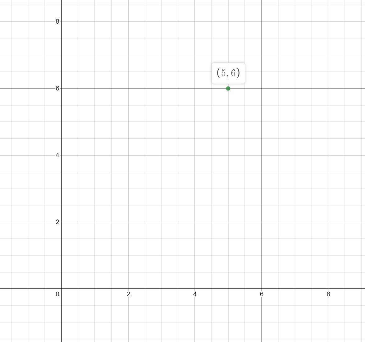
Complex numbers can be written as \(a + bi\), where \(a\) is the real part, and \(b\) is the imaginary part. Each complex number can be thought as a point on the complex plane. The complex plane is just a cartesian plane, where the x axis represents real numbers, and the y axis represents complex numbers. Graphing points is simple: just treat \(a\) as an x value, and \(b\) as a y value. So, \(5 + 6i\) can be graphed as so:

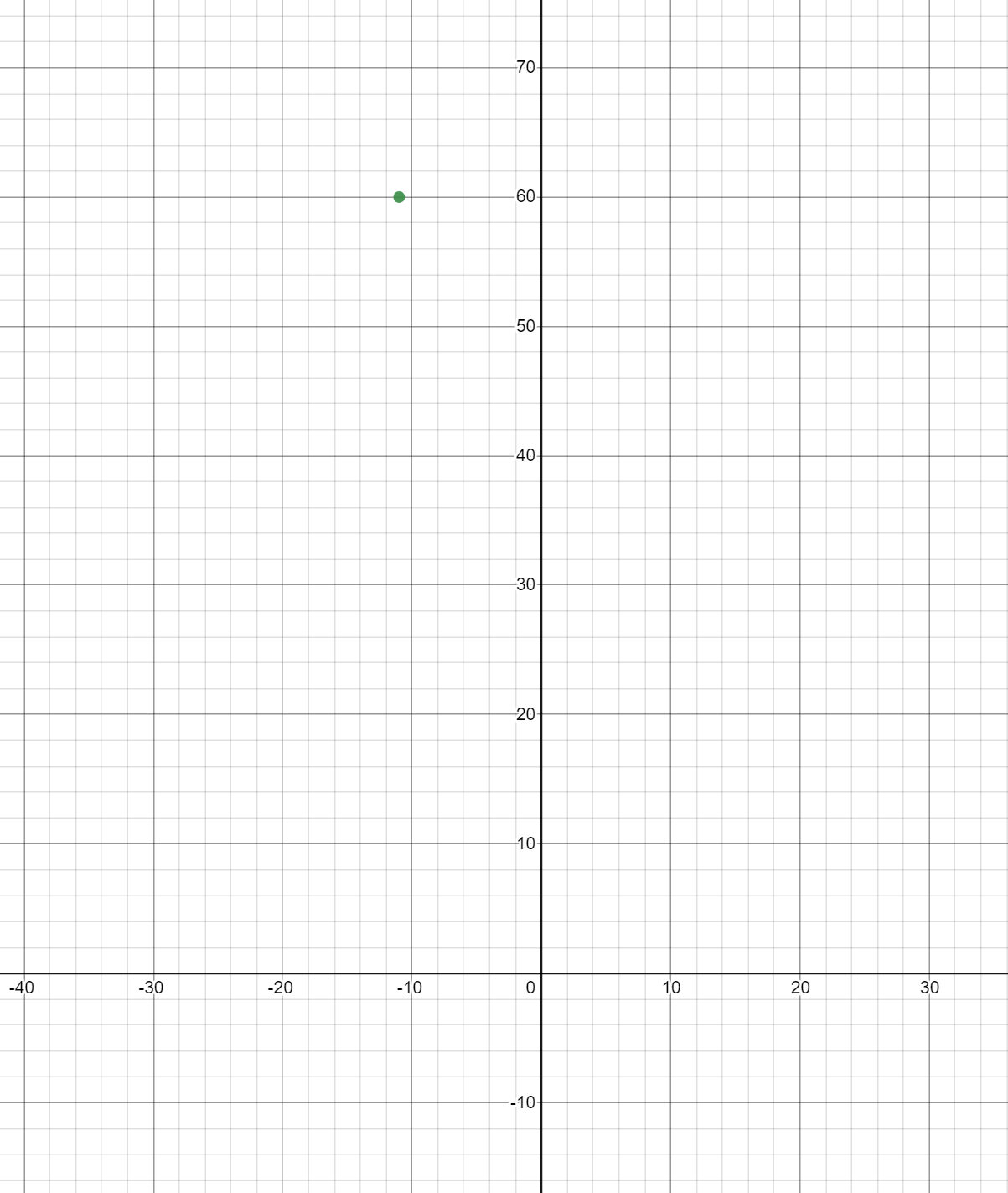
The cool thing with the complex plane is that you can do operations on each point, and you can get different points in return. For example, if we square the point graphed above, we will get a different point. However, squaring a point isn’t as easy as squaring the a and b values separately. Like binomials, we must use the distributive property when multiplying. So, we have:

Notice how when we squared \(i\), we got \(-1\). That’s just a consequence of the identity discussed earlier. \(i^2 = -1\). Now, our point can be graphed as so:

I also mentioned earlier that we can use newton’s method on complex functions. For example, take the function \(f(z) = z^3 + 1\). Just so we can check our answers, let’s solve for the roots first. We have:

Now that we know the roots, let’s use newton’s method. We’ll start at, say, \(z_0=2\). We have:

Towards the end, I stopped showing the process, but I just did the same thing over and over again. Using this method, we can approximate the root, starting at any point on the complex plane! (Except, of course, the critical points of the function, one of which happens to be at \(z=0 + 0i\), since \(3z^2 = 0\))

You may be wondering, “how can I make a fractal using this information?” Well, that is a great question! Recall that newton’s method will give a root, since we have no way of specifying exactly which root we want. We will see that we can, in fact, see which groups of numbers converge to which groups using newton’s method, but only once we graph which numbers converge to which groups.

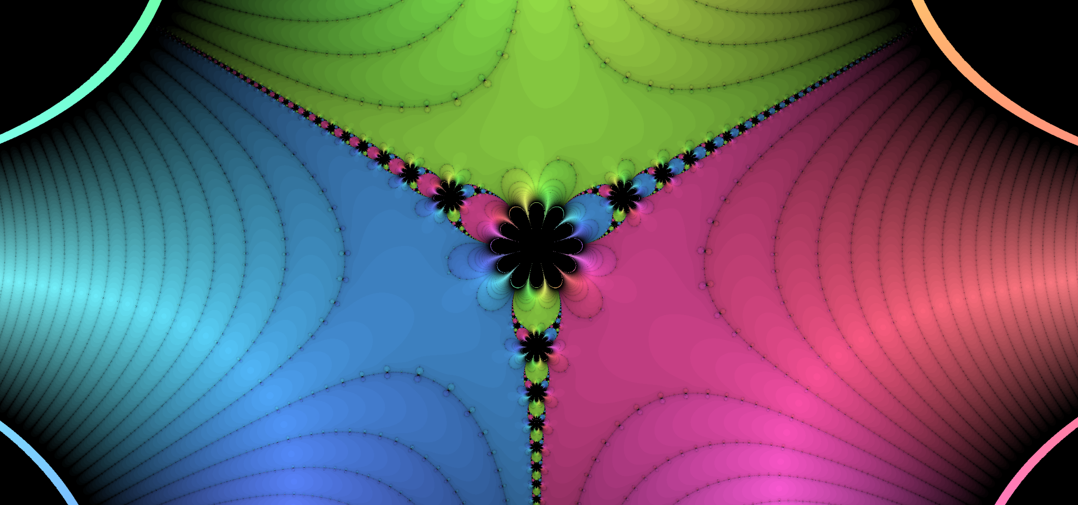
To show you, I’ll make a graph of the complex plane, where I use newton’s method with function \(f(z) = z^3 + 1\) on each point. If newton’s method converges to \(-1 + 0 i\), I’ll color the point red, if it converges to \(\dfrac{1}{2} + \dfrac{\sqrt3}{2} i\), I’ll color the point green, and if it converges to \(\dfrac{1}{2} - \dfrac{\sqrt3}{2} i\), I’ll color the point blue. Take a look:

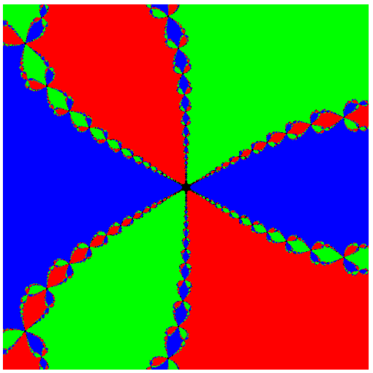
Wow, a fractal! Yes, making fractals are as simple as that.

Including Complex Numbers in Code

Unfortunately, javascript (unlike python) doesn’t have a built-in version of complex numbers for us to use, do we’ll have to make our own. Since there are 2 elements to each complex number–the real and imaginary parts–we can just use an array to store each complex number. (I would use a tuple if they existed in javascript, but alas…) Let’s edit our code to reflect that:

function newtonsMethod(f, fp, x0, steps) {
  let xn = x0;
  for (let n = 0; n < steps; n++) {
    xn = complex_sub(xn, complex_div(f(xn), fp(xn)))
  }
  return xn
}

console.log("Output:",
  newtonsMethod(
    x => complex_sub(complex_pow(x, 2), 1),
    x => complex_mul(x, 2),
    [-15, 0],
    10
  )
)

Notice how I replaced all mathematical operations with functions. Why is that? Well, try multiplying arrays in javascript, or raising them to a power, or subtracting them:

>> [1, 2] ** 2
NaN

>> [1, 2] * 2
NaN

>> [3, 4] - [1, 2]
NaN

As you can see, we never get the answer we want! We always get NaN, which stands for “Not a Number”. When javascript tries to perform a mathematical operation, it takes both arguments, in this case, the array and the number, (or another array), and sees that they aren’t compatible. It’s like trying to divide a banana by an apple. It’s not immediately obvious how one could go about such a task, although one could infer… However, javascript isn’t smart enough to infer that, so we have to define it ourselves. Hence the new complex_... functions.

Writing them should be easy, we just need to figure out how each complex operation affects the real and imaginary parts of the variable. Let’s start with complex subtraction:

Similarly, addition can be proved as so:

Okay, those were simple. We just use the distributive property on the minus/plus, and group up the real and imaginary parts. What about multiplication and division?

Multiplication was also relatively easy, I just used the distributive property to multiply the binomials, I used the imaginary identity, and last I just grouped up the numbers again according to their “imaginary-ness”. This last one, complex exponents, is probably the most interesting, as it makes use of Euler’s formula, and the polar form of complex numbers. Blackpenredpen has a great video on this proof

Now, we can easily convert these formulas into code using lambda functions:

const complex_mul = ([a, b], [c, d]) => [a*c - b*d, a*d + b*c]
const complex_sub = ([a, b], [c, d]) => [a-c, b-d]
const complex_add = ([a, b], [c, d]) => [a+c, b+d]
const complex_sqdist = ([a, b], [c, d]) => (a-c)**2 + (b-d)**2

const complex_div = ([a, b], [c, d]) => {
  let den = c**2 + d**2
  return [(a*c+b*d)/den, (b*c-a*d)/den]
}

const complex_pow = ([a, b], [c, d]) => {
  let r = Math.sqrt(a**2 + b**2)
  let theta = Math.atan2(b, a)
  let x = r**c * Math.exp(-d * theta)
  let y = c * theta + d * Math.log(r)
  return [x * Math.cos(y), x * Math.sin(y)]
}

Note: I added a function complex_sqdist, which just computes the squared euclidian distance between 2 complex points. It’s pretty much just the pythagorean theorem. The reason why I keep it squared instead of taking the square root is because square root is one of the most computationally intensive mathematical operations, meaning it takes the most time to compute. If we just leave it out, we can use that time to calculate other points! Double note: The only place I use it is when I check if a point converges to a root.

Now, we can make a quick version of the newton’s fractal using the canvas. I’ll use the following code to create a canvas, then go over every pixel with newton’s method, then color it according to its root.

index.html

<!DOCTYPE html>
<html lang="en">
  <head>
    <meta charset="UTF-8" />
    <meta http-equiv="X-UA-Compatible" content="IE=edge" />
    <meta name="viewport" content="width=device-width, initial-scale=1.0" />
    <title>Document</title>
    <script src="complexfunctions.js"></script>
  </head>
  <body>
    <canvas width="500" height="500" id="canvas"></canvas>

    <script>
      // Initialize canvas context
      let c = document.getElementById("canvas");
      let ctx = c.getContext("2d");

      // Define f(x) and f'(x)
      let f = (x) => complex_add(complex_pow(x, [3, 0]), [1, 0]);
      let fp = (x) => complex_mul([3, 0], complex_pow(x, [2, 0]));

      // Loop through every pixel
      for (let x = 0; x < c.width; x++) {
        for (let y = 0; y < c.height; y++) {

          // Map the position elements from [0, 500] to [-1, 1]
          let pos = [
            (x - c.width / 2) / c.height,
            (y - c.height / 2) / c.height,
          ];

          // Perform newton's method on the position
          let convergingRoot = newtonsMethod(f, fp, pos, 20);

          // Set color based on root it diverges to
          if (complex_sqdist(convergingRoot, [0.5, 0.866]) <= 0.1) {
            ctx.fillStyle = "rgb(255, 0, 0)";
          } else if (complex_sqdist(convergingRoot, [0.5, -0.866]) <= 0.1) {
            ctx.fillStyle = "rgb(0, 255, 0)";
          } else if (complex_sqdist(convergingRoot, [-1, 0]) <= 0.1) {
            ctx.fillStyle = "rgb(0, 0, 255)";
          } else {
            // Make it black if it diverges/doesn't converge quick enough
            ctx.fillStyle = "rgb(0, 0, 0)"
          }

          // Draw the pixel
          ctx.fillRect(x, y, 1, 1);
        }
      }
    </script>
  </body>
</html>

complexfunctions.js

const complex_mul = ([a, b], [c, d]) => [a*c - b*d, a*d + b*c]
const complex_sub = ([a, b], [c, d]) => [a-c, b-d]
const complex_add = ([a, b], [c, d]) => [a+c, b+d]
const complex_sqdist = ([a, b], [c, d]) => (a-c)**2 + (b-d)**2

const complex_div = ([a, b], [c, d]) => {
  let den = c**2 + d**2
  return [(a*c+b*d)/den, (b*c-a*d)/den]
}

const complex_pow = ([a, b], [c, d]) => {
  let r = Math.sqrt(a**2 + b**2)
  let theta = Math.atan2(b, a)
  let x = r**c * Math.exp(-d * theta)
  let y = c * theta + d * Math.log(r)
  return [x * Math.cos(y), x * Math.sin(y)]
}

function newtonsMethod(f, fp, x0, steps) {
  let xn = x0;
  for (let i = 0; i < steps; i++) {
    xn = complex_sub(xn, complex_div(f(xn), fp(xn)))
  }
  return xn
}

And now, if you run this page on your browser, after waiting a couple seconds, in front of you is a newton fractal of your own!

Other things

You may notice that the newton fractal you just created takes a long time to render a single frame versus the one I made. That’s because you use the CPU to calculate every pixel. In your computer, there are a couple ways you can make a calculation. The first way is through the CPU, which is really good at executing complex instructions. Another option is through the GPU, which is really good at executing simple instructions, at ton of times over, at the same time.

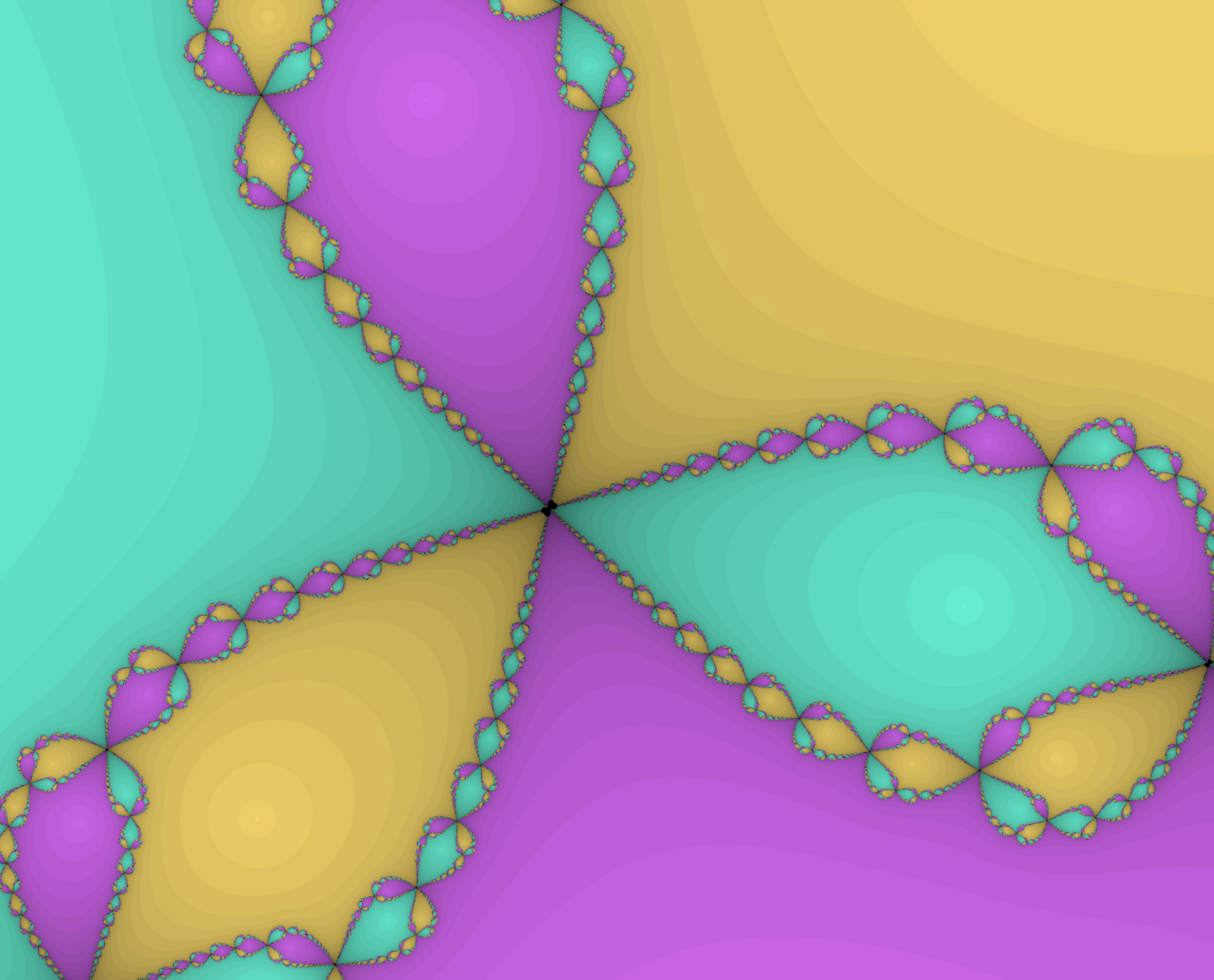
WebGL2 is a way to harness the power of your GPU, and it allows newton’s method to be sped up to a rate at which you can hardly notice the rendering time! This is what I use on my version, and writing the code for it is slightly different. However, I won’t be getting into that in this blog post, since it is a whole other topic and deserves its own post.

Another thing you may notice is that you can just type in a math expression on my newton fractal, instead of typing out all the complex functions to replicate the equation in code. That’s because I made my own lexer, parser, and compiler in order to take a mathematical expression and turn it into GLSL code to run on the GPU. It currently isn’t that good–I rushed it in order to have a finished version of my fractal working, and I haven’t had time to make it more efficient.

Parsers, Lexers, and Compilers are also very complicated and deserve their own post to fully do them justice.

Some time in the future, I will get around to making them, but for now, enjoy the fractals! Thanks for reading!

$$